Many modern machine learning algorithms have a large number of hyperparameters. To effectively use these algorithms, we need to pick good hyperparameter values.
In this article, we talk about Bayesian Optimization, a suite of techniques often used to tune hyperparameters. More generally, Bayesian Optimization can be used to optimize any black-box function.
许多现代机器学习算法具有大量超参数。为了有效地使用这些算法,我们需要选择良好的超参数值。在本文中,我们讨论贝叶斯优化,这是一套经常用于调整超参数的技术。更一般地说,贝叶斯优化可用于优化任何黑盒函数。
Mining Gold! 黄金开采!
Let us start with the example of gold mining. Our goal is to mine for gold in an unknown land
在这里,Krige 教授使用高斯过程对金的浓度进行建模。
让我们从黄金开采的例子开始。我们的目标是在一片未知的土地上开采黄金
1
有趣的是,我们的例子类似于高斯过程(也称克里金)的首次运用之一。.
For now, we assume that the gold is distributed about a line. We want to find the location along this line with the maximum gold while only drilling a few times (as drilling is expensive).
目前,我们假设黄金分布在一条线周围。我们希望找到沿着这条线的最大黄金位置,同时只需钻几次(因为钻探成本高昂)。
Let us suppose that the gold distribution looks something like the function below. It is bi-modal, with a maximum value around . For now, let us not worry about the X-axis or the Y-axis units.
让我们假设金子分布 看起来类似下面的函数。它是双峰的,最大值大约在 附近。目前,让我们不担心 X 轴或 Y 轴的单位。

Initially, we have no idea about the gold distribution. We can learn the gold distribution by drilling at different locations. However, this drilling is costly. Thus, we want to minimize the number of drillings required while still finding the location of maximum gold quickly.
最初,我们对金子分布一无所知。我们可以通过在不同位置钻探来了解金子分布。然而,这种钻探是昂贵的。因此,我们希望尽量减少所需的钻探次数,同时迅速找到最大金子位置。
We now discuss two common objectives for the gold mining problem.
现在我们讨论金矿问题的两个常见目标。
-
Problem 1: Best Estimate of Gold Distribution (Active Learning)
问题 1:金子分布的最佳估计(主动学习)
In this problem, we want to accurately estimate the gold distribution on the new land. We can not drill at every location due to the prohibitive cost. Instead, we should drill at locations providing high information about the gold distribution. This problem is akin to Active Learning
在这个问题中,我们希望准确估计新土地上的金分布。由于成本过高,我们无法在每个地点钻探。相反,我们应该在提供关于金分布的高信息量的地点钻探。这个问题类似于主动学习。. -
Problem 2: Location of Maximum Gold (Bayesian Optimization)
问题 2: 最大黄金位置(贝叶斯优化)
In this problem, we want to find the location of the maximum gold content. We, again, can not drill at every location. Instead, we should drill at locations showing high promise about the gold content. This problem is akin to Bayesian Optimization
在这个问题中,我们希望找到最大黄金含量的位置。同样,我们无法在每个地点钻探。相反,我们应该在显示出对黄金含量有很高希望的地点钻探。这个问题类似于贝叶斯优化。.
We will soon see how these two problems are related, but not the same.
我们很快会看到这两个问题如何相关,但并不相同。
Active Learning 主动学习
For many machine learning problems, unlabeled data is readily available. However, labeling (or querying) is often expensive. As an example, for a speech-to-text task, the annotation requires expert(s) to label words and sentences manually. Similarly, in our gold mining problem, drilling (akin to labeling) is expensive.
对于许多机器学习问题,未标记的数据是 readily available。然而,标记(或查询)往往很昂贵。例如,对于语音转文本的任务,注释需要专家手动标记单词和句子。同样,在我们的金矿问题中,打孔(类似于标记)很昂贵。
Active learning minimizes labeling costs while maximizing modeling accuracy. While there are various methods in active learning literature, we look at uncertainty reduction. This method proposes labeling the point whose model uncertainty is the highest. Often, the variance acts as a measure of uncertainty.
主动学习减少标记成本,同时最大化建模准确性。虽然主动学习文献中有各种方法,我们关注不确定性减少。该方法建议标记模型不确定性最高的点。通常,方差充当不确定性的度量。
Since we only know the true value of our function at a few points, we need a surrogate model for the values our function takes elsewhere. This surrogate should be flexible enough to model the true function. Using a Gaussian Process (GP) is a common choice, both because of its flexibility and its ability to give us uncertainty estimates
Please find this amazing video from Javier González on Gaussian Processes.
请查看哈维尔·冈萨雷斯关于高斯过程的精彩视频。
由于我们只在一些点上知道我们函数的真实值,我们需要一个替代模型来代表函数在其他地方取值。这个替代模型应该足够灵活,可以模拟真实函数。使用高斯过程(GP)是一个常见的选择,因为它既灵活,又能给出不确定性的估计。高斯过程支持通过使用特定的核函数和均值函数来设置先验。你可能会对这篇出色的 Distill 文章感兴趣。.
Our surrogate model starts with a prior of — in the case of gold, we pick a prior assuming that it’s smoothly distributed
我们的替代模型从 的先验开始——以黄金为例,我们选择假设其呈平滑分布
3
细节:我们使用 Matern 5/2 核,因其偏爱具有二阶可微性质的函数。有关 Matern 核的详细信息,请参阅 Rasmussen 和 Williams 2004 年的著作以及 scikit-learn。随着我们评估点(钻探),我们会获得更多数据供替代模型进行学习,并根据贝叶斯法则进行更新。

每个新数据点更新我们的替代模型,使其更接近真实情况。黑线和灰色阴影区域表示在钻探前后我们对金属分布估计的均值 和不确定性 。
In the above example, we started with uniform uncertainty. But after our first update, the posterior is certain near and uncertain away from it. We could just keep adding more training points and obtain a more certain estimate of .
在上面的例子中,我们从均匀不确定性开始。但在我们的第一个更新后,后验在 附近是确定的,在离其远的地方是不确定的。我们可以继续添加更多训练点,并获得对 更确定的估计。
However, we want to minimize the number of evaluations. Thus, we should choose the next query point “smartly” using active learning. Although there are many ways to pick smart points, we will be picking the most uncertain one.
但是,我们希望最小化评估次数。因此,我们应该使用主动学习“聪明地”选择下一个查询点。虽然有许多方法可以选择聪明的点,但我们将选择最不确定的点。
This gives us the following procedure for Active Learning:
这给我们提供了主动学习的以下步骤:
- Choose and add the point with the highest uncertainty to the training set (by querying/labeling that point)
选择并将具有最高不确定性的点添加到训练集中(通过查询/标记该点) - Train on the new training set
对新的训练集进行训练 - Go to #1 till convergence or budget elapsed
转到#1,直至收敛或耗尽预算
Let us now visualize this process and see how our posterior changes at every iteration (after each drilling).
现在让我们可视化这个过程,并看看我们的后验在每次迭代(每次钻孔后)后如何变化。

The visualization shows that one can estimate the true distribution in a few iterations. Furthermore, the most uncertain positions are often the farthest points from the current evaluation points. At every iteration, active learning explores the domain to make the estimates better.
该可视化显示,人们可以在几次迭代中估计真实分布。此外,最不确定的位置通常是当前评估点的最远处。在每次迭代中,主动学习会探索领域以改进估计值。
Bayesian Optimization 贝叶斯优化
In the previous section, we picked points in order to determine an accurate model of the gold content. But what if our goal is simply to find the location of maximum gold content? Of course, we could do active learning to estimate the true function accurately and then find its maximum. But that seems pretty wasteful — why should we use evaluations improving our estimates of regions where the function expects low gold content when we only care about the maximum?
在前一节中,我们选择了一些点,以便确定金含量的准确模型。但是,如果我们的目标只是为了找到最大金含量的位置呢?当然,我们可以进行主动学习来准确估计真正的函数,然后找到它的最大值。但这似乎相当浪费 — 为什么我们要在我们只关心最大值的地方改善估计函数期望低金含量的地区呢?
This is the core question in Bayesian Optimization: “Based on what we know so far, which point should we evaluate next?” Remember that evaluating each point is expensive, so we want to pick carefully! In the active learning case, we picked the most uncertain point, exploring the function. But in Bayesian Optimization, we need to balance exploring uncertain regions, which might unexpectedly have high gold content, against focusing on regions we already know have higher gold content (a kind of exploitation).
这是贝叶斯优化中的核心问题:“根据我们目前所知,我们应该评估哪个点?”请记住,评估每个点都是昂贵的,所以我们需要谨慎选择!在主动学习的情况下,我们选择了最不确定的点,来探索函数。但是在贝叶斯优化中,我们需要平衡对探索不确定区域(可能意外拥有高含金量)的关注,与对已知含金量较高区域的关注(一种开发利用)之间的关系。
We make this decision with something called an acquisition function. Acquisition functions are heuristics for how desirable it is to evaluate a point, based on our present model
我们通过一个称为收购函数的东西做出这个决定。收购函数是根据我们当前的模型评估一个点的可取性的启发式算法
4
有关收购函数的更多细节可在此链接获取。我们将在本节大部分时间内讨论不同的收购函数选项。
This brings us to how Bayesian Optimization works. At every step, we determine what the best point to evaluate next is according to the acquisition function by optimizing it. We then update our model and repeat this process to determine the next point to evaluate.
这使我们了解到贝叶斯优化的工作原理。在每一步,我们通过优化收购函数确定下一个评估点。然后我们更新我们的模型并重复此过程以确定下一个要评估的点。
You may be wondering what’s “Bayesian” about Bayesian Optimization if we’re just optimizing these acquisition functions. Well, at every step we maintain a model describing our estimates and uncertainty at each point, which we update according to Bayes’ rule
你可能会想知道如果我们只是优化这些收购函数,那么贝叶斯优化中的“贝叶斯”是什么。好吧,每一步我们维护一个描述我们在每个点的估计和不确定性的模型,根据贝叶斯定理我们更新它。
在每一步,我们的收购函数都是基于这个模型的,如果没有它们,什么都不可能!
Formalizing Bayesian Optimization
贝叶斯优化的形式化
Let us now formally introduce Bayesian Optimization. Our goal is to find the location () corresponding to the global maximum (or minimum) of a function .
We present the general constraints in Bayesian Optimization and contrast them with the constraints in our gold mining example现在让我们正式介绍贝叶斯优化。我们的目标是找到与函数 的全局最大值(或最小值)对应的位置( )。我们介绍贝叶斯优化中的一般约束,并将其与我们的金矿开采示例中的约束进行对比 5 。以下部分基于 Uber 的 Peter Fraizer 关于贝叶斯优化的幻灯片/演讲内容:.
General Constraints 一般约束 |
Constraints in Gold Mining example |
|---|---|
| ’s feasible set is simple,
e.g., box constraints. 的可行集 很简单,例如,箱式约束。 |
Our domain in the gold mining problem is a single-dimensional box constraint: . 在黄金采矿问题中,我们的定义域是一个单维度的箱式约束: 。 |
| is continuous but lacks special structure,
e.g., concavity, that would make it easy to optimize. 是连续的,但缺乏特殊结构,例如凹凸性,这使得优化变得困难。 |
Our true function is neither a convex nor a concave function, resulting in local optimums. 我们的真实函数既不是凸函数也不是凹函数,导致局部最优解。 |
| is derivative-free:
evaluations do not give gradient information. 是无导数的:评估不提供梯度信息。 |
Our evaluation (by drilling) of the amount of gold content at a location did not give us any gradient information. 我们通过钻探对某一地点的金含量进行的评估没有提供任何梯度信息。 |
| is expensive to evaluate:
the number of times we can evaluate it
is severely limited. 的评估成本很高:我们能够对其进行评估的次数严重受限。 |
Drilling is costly. 钻探成本高昂。 |
| may be noisy. If noise is present, we will assume it is independent and normally distributed, with common but unknown variance. 可能存在噪音。如果存在噪音,我们将假设其独立且服从正态分布,具有常见但未知的方差。 |
We assume noiseless measurements in our modeling (though, it is easy to incorporate normally distributed noise for GP regression). 在我们的建模中假设无噪声的测量(尽管很容易将正态分布噪声纳入 GP 回归)。 |
To solve this problem, we will follow the following algorithm:
为解决这一问题,我们将遵循以下算法:
-
We first choose a surrogate model for modeling the true function and define its prior.
我们首先选择一个代理模型来对真实函数 进行建模,并定义其先验。 -
Given the set of observations (function evaluations), use Bayes rule to obtain the posterior.
针对给定的观察集合(函数评估),使用贝叶斯规则来获得后验函数。 -
Use an acquisition function , which is a function of the posterior, to decide the next sample point .
使用一个收购函数 ,它是后验函数的一个函数,来决定下一个样本点 。 -
Add newly sampled data to the set of observations and goto step #2 till convergence or budget elapses.
将新采样数据添加到观察集合中,并进行步骤 #2 直到收敛或预算耗尽。
Acquisition Functions 获取函数
Acquisition functions are crucial to Bayesian Optimization, and there are a wide variety of options
收集函数对贝叶斯优化至关重要,有各种各样的选择
6
请查阅华盛顿大学圣路易斯分校的这些幻灯片以了解更多有关收集函数的内容。在接下来的部分中,我们将介绍多种选择,并提供直觉和示例。
Probability of Improvement (PI)
改善的概率(PI)
This acquisition function chooses the next query point as the one which has the highest probability of improvement over the current max . Mathematically, we write the selection of next point as follows,
此获取函数选择下一个查询点,该点具有在当前最大 上的改进概率最高。从数学上讲,我们将下一个点的选择写为以下形式,
where, 其中,
- indicates probability
表示概率 - is a small positive number
是一个小的正数 - And, where is the location queried at time step.
而且, 其中 是在 时间步进行查询的位置。
Looking closely, we are just finding the upper-tail probability (or the CDF) of the surrogate posterior. Moreover, if we are using a GP as a surrogate the expression above converts to,
仔细观察,我们只是在寻找代理后验的上尾概率(或者累积分布函数)。此外,如果我们使用高斯过程作为代理,上述表达式转换为:
where, 其中,
- indicates the CDF 表示累积分布函数
The visualization below shows the calculation of . The orange line represents the current max (plus an ) or . The violet region shows the probability density at each point. The grey regions show the probability density below the current max. The “area” of the violet region at each point represents the “probability of improvement over current maximum”. The next point to evaluate via the PI criteria (shown in dashed blue line) is .
下面的可视化展示了 的计算。橙色线表示当前最大值(加上 )或 。紫色区域显示了每个点的概率密度,灰色区域显示了当前最大值以下的概率密度。紫色区域在每个点的“面积”表示“改善当前最大值的概率”。根据 PI 准则(以虚线蓝线显示),下一个要通过 PI 准则评估的点是 。

Intuition behind in PI
对 PI 中 的直觉
PI uses to strike a balance between exploration and exploitation.
Increasing results in querying locations with a larger as their probability density is spread.
PI 使用 来在探索和开发之间取得平衡。增加 会导致查询具有更大 的位置,因为它们的概率密度被扩散。
Let us now see the PI acquisition function in action. We start with .
现在让我们看看 PI 获取函数的运作。我们从 开始。

Looking at the graph above, we see that we reach the global maxima in a few iterations
观察上面的图表,我们看到在少数迭代中达到全局极值
7
。平局被随机打破...在前几次迭代
8
中,我们的代理具有较大的不确定性 。不确定性的比例由灰色半透明区域识别。收获函数最初利用具有很高承诺的区域
9
。当前极值附近的点,这导致该地区的不确定性很高 。这一观察还表明,我们不需要构建对黑盒函数的准确估计,即可找到其最大值。

The visualization above shows that increasing to 0.3, enables us to explore more. However, it seems that we are exploring more than required.
上面的可视化显示,将 增加到 0.3,可以让我们更多地探索。然而,看起来我们探索的超过了所需的范围。
What happens if we increase a bit more?
如果我们再增加 会发生什么?

We see that we made things worse! Our model now uses , and we are unable to exploit when we land near the global maximum. Moreover, with high exploration, the setting becomes similar to active learning.
我们发现我们让事情变得更糟了!我们的模型现在使用 ,而且当我们接近全局最大值时,我们无法进行利用。而且,高探索度使得情况类似于积极学习。
Our quick experiments above help us conclude that controls the degree of exploration in the PI acquisition function.
我们上述的快速实验有助于我们得出结论: 控制了 PI 获取函数中的探索程度。
Expected Improvement (EI)
期望改进(EI)
Probability of improvement only looked at how likely is an improvement, but, did not consider how much we can improve. The next criterion, called Expected Improvement (EI), does exactly that
改进概率只关注改进的可能性,但并未考虑我们可以改进多少。下一个标准叫做期望改进(EI),确切地做到了这一点
10
。关于期望改进获取函数的良好介绍可参见 Thomas Huijskens 的这篇帖子以及 Peter Frazier 的这些幻灯片!其理念相当简单——选择下一个查询点,其在当前最大 之上具有最高的期望改进,其中 和 是在 时间步骤处进行查询的位置。
In this acquisition function, query point, , is selected according to the following equation.
在此获取功能中, 查询点 根据以下方程式被选择。
Where, is the actual ground truth function, is the posterior mean of the surrogate at timestep, is the training data and is the actual position where takes the maximum value.
其中, 是实际的基本真实函数, 是 时间步骤处替代模型的后验均值, 是训练数据 , 而 是 取得最大值的实际位置。
In essence, we are trying to select the point that minimizes the distance to the objective evaluated at the maximum. Unfortunately, we do not know the ground truth function, . Mockus
本质上,我们试图选择使目标函数在最大值处评估的距离最小化的点。不幸的是,我们不知道基本真实函数 。Mockus
提出了以下采集函数以克服这个问题。
where is the maximum value that has been encountered so far. This equation for GP surrogate is an analytical expression shown below.
其中 是迄今为止遇到的最大值。高斯过程替代模型的这个方程是下面所示的解析表达式。
where indicates CDF and indicates pdf.
其中 表示累积分布函数(CDF), 表示概率密度函数(PDF)。
From the above expression, we can see that Expected Improvement will be high when: i) the expected value of is high, or, ii) when the uncertainty around a point is high.
根据上述表达式,我们可以看到,当:i) 的期望值较高时,或者,ii)在一个点周围的不确定性 较高时,预期改善将会很大。
Like the PI acquisition function, we can moderate the amount of exploration of the EI acquisition function by modifying .
与 PI 采集函数类似,我们可以通过修改 来调节 EI 采集函数的探索量。

For we come close to the global maxima in a few iterations.
在 中,我们在几次迭代中接近全局极大值。
We now increase to explore more.
现在我们增加 以进行更多探索。

As we expected, increasing the value to makes the acquisition function explore more. Compared to the earlier evaluations, we see less exploitation. We see that it evaluates only two points near the global maxima.
正如我们预期的那样,增加值到 会使获取函数进行更多探索。与之前的评估相比,我们看到少了一些开发。我们发现它只评估了全局极大值附近的两个点。
Let us increase even more.
让我们进一步增加 。

Is this better than before? It turns out a yes and a no; we explored too much at and quickly reached near the global maxima. But unfortunately, we did not exploit to get more gains near the global maxima.
这比以前好吗?结果是肯定和否定的;我们在 处探索得太多,很快就接近了全局最大值。但不幸的是,我们没有充分利用以获得更多的收益。
PI vs Ei
We have seen two closely related methods, The Probability of Improvement and the Expected Improvement.
我们看到了两种密切相关的方法,改进的概率和期望改进。

The scatter plot above shows the policies’ acquisition functions evaluated on different points
Thompson Sampling 汤普森抽样
Another common acquisition function is Thompson Sampling
另一个常见的收获函数是汤普森抽样。
在每一步,我们从替代后验中抽样一个函数并对其进行优化。例如,在金矿开采的情况下,我们会对产出的概率分布进行抽样,并在其峰值处进行评估(钻探)。
Below we have an image showing three sampled functions from the learned surrogate posterior for our gold mining problem. The training data constituted the point and the corresponding functional value.
下面是一幅图像,显示了我们在黄金采矿问题上学习的替代后验的三个样本函数。训练数据包括点 及其对应的函数值。

We can understand the intuition behind Thompson sampling by two observations:
通过两点观察我们可以理解 Thompson 采样的直觉:
-
Locations with high uncertainty () will show a large variance in the functional values sampled from the surrogate posterior. Thus, there is a non-trivial probability that a sample can take high value in a highly uncertain region. Optimizing such samples can aid exploration.
在不确定性较高的地方( )将会在从替代后验中抽样的函数值中显示出较大的方差。因此,有相当大的概率一个样本可以在高度不确定的地区获得较高的值。优化这样的样本可以促进探索。As an example, the three samples (sample #1, #2, #3) show a high variance close to . Optimizing sample 3 will aid in exploration by evaluating .
例如,三个样本(样本 #1, #2, #3)在 附近显示出较大的方差。对样本 3 的优化将通过评估 有助于探索。 -
The sampled functions must pass through the current max value, as there is no uncertainty at the evaluated locations. Thus, optimizing samples from the surrogate posterior will ensure exploiting behavior.
抽样的函数必须通过当前最大值,因为在评估的地点没有不确定性。因此,从替代后验中优化样本将确保利用行为。As an example of this behavior, we see that all the sampled functions above pass through the current max at . If were close to the global maxima, then we would be able to exploit and choose a better maximum.
作为这种行为的例子,我们可以看到以上所有采样函数都通过了当前的最大值 。如果 接近全局最大值,那么我们就能够利用并选择更好的最大值。

The visualization above uses Thompson sampling for optimization. Again, we can reach the global optimum in relatively few iterations.
上面的可视化使用了汤普森抽样进行优化。同样,我们可以在相对较少的迭代中达到全局最优解。
Random 随机
We have been using intelligent acquisition functions until now.
We can create a random acquisition function by sampling
randomly.
直到现在,我们一直在使用智能采集函数。我们可以通过随机抽样 来创建一个随机采集函数。

The visualization above shows that the performance of the random acquisition function is not that bad! However, if our optimization was more complex (more dimensions), then the random acquisition might perform poorly.
上面的可视化显示,随机获取函数的性能并不那么差!然而,如果我们的优化更复杂(维度更多)那么随机获取可能表现不佳。
Summary of Acquisition Functions
收购功能摘要
Let us now summarize the core ideas associated with acquisition functions: i) they are heuristics for evaluating the utility of a point; ii) they are a function of the surrogate posterior; iii) they combine exploration and exploitation; and iv) they are inexpensive to evaluate.
现在让我们总结与收购功能相关的核心思想:i)它们是评估点效用的启发式方法;ii)它们是替代后验的函数;iii)它们结合了探索和利用;iv)它们的评估成本低廉。
Other Acquisition Functions
其他收购功能
We have seen various acquisition functions until now. One trivial way to come up with acquisition functions is to have a explore/exploit combination.
目前我们已经看到各种收购功能。提出收购功能的一个简单方法是采用探索/利用组合方式。
Upper Confidence Bound (UCB)
上置信界限(UCB)
One such trivial acquisition function that combines the exploration/exploitation tradeoff is a linear combination of the mean and uncertainty of our surrogate model. The model mean signifies exploitation (of our model’s knowledge) and model uncertainty signifies exploration (due to our model’s lack of observations).
一个结合探索/开发权衡的微不足道的收购功能是我们替代模型均值和不确定性的线性组合。模型均值表示利用(我们模型的知识),而模型不确定性表示探索(由于我们模型缺乏观察)。
The intuition behind the UCB acquisition function is weighing of the importance between the surrogate’s mean vs. the surrogate’s uncertainty. The above is the hyperparameter that can control the preference between exploitation or exploration.
UCB 收购功能背后的直觉是权衡替代的平均值与替代的不确定性之间的重要性。上述 是可以控制开发或探索偏好的超参数。
We can further form acquisition functions by combining the existing acquisition functions though the physical interpretability of such combinations might not be so straightforward. One reason we might want to combine two methods is to overcome the limitations of the individual methods.
我们可以通过结合现有的获取函数来进一步形成获取功能,尽管这种组合的物理可解释性可能并不那么直观。我们希望结合两种方法的一个原因是为了克服各个方法的局限性。
Probability of Improvement + Expected Improvement (EI-PI)
改进概率 + 预期改进 (EI-PI)
One such combination can be a linear combination of PI and EI.
We know PI focuses on the probability of improvement, whereas EI focuses on the expected improvement. Such a combination could help in having a tradeoff between the two based on the value of .
其中一种组合可以是 PI 和 EI 的线性组合。我们知道 PI 侧重于改进的概率,而 EI 侧重于预期改进。这样的组合可以根据 的值在两者之间取得权衡。
Gaussian Process Upper Confidence Bound (GP-UCB)
高斯过程上置信界限 (GP-UCB)
Before talking about GP-UCB, let us quickly talk about regret. Imagine if the maximum gold was units, and our optimization instead samples a location containing units, then our regret is
. If we accumulate the regret over iterations, we get what is called cumulative regret.
在讨论 GP-UCB 之前,让我们快速谈谈遗憾。想象一下,如果最大黄金量为 个单位,而我们的优化反而对包含 单位的位置进行抽样,那么我们的遗憾就是 。如果我们在 次迭代中累积遗憾,就得到了所谓的累积遗憾。
GP-UCB’s GP-UCB 的
公式的表示如下:
Where is the timestep.
其中 是时间步长。
Srinivas et. al. Srinivas 等人
开发了一个时间表 ,他们在理论上证明了最小化累积遗憾。
Comparison 对比
We now compare the performance of different acquisition functions on the gold mining problem
我们目前对黄金开采问题上不同收获函数的表现进行比较
14
要了解更多关于收获函数之间的差异,请查看 Nando De Freitas 的这些精彩幻灯片。我们已经为每个收获函数使用最佳的超参数。我们多次使用不同种子运行了随机收获函数,并绘制了每次迭代时感知到的黄金的平均值。

The random strategy is initially comparable to or better than other acquisition functions
随机策略最初与其他收获函数相当或更好
15
UCB 和 GP-UCB 已在可折叠部分中提到。然而,随机策略感知到的最大黄金增长缓慢。相比之下,其他收获函数可以在少量迭代中找到一个好的解决方案。事实上,大多数收获函数在仅三次迭代中就接近全局最大值。
Hyperparameter Tuning 超参数调优
Before we talk about Bayesian optimization for hyperparameter tuning
在我们讨论贝叶斯优化用于超参数调优之前
在接下来的讨论中,我们将快速区分超参数和参数:超参数是在学习之前设置的,而参数是从数据中学习得到的。为了说明这种区别,我们以岭回归的例子来说明。
In Ridge regression, the weight matrix is the parameter, and the regularization coefficient is the hyperparameter.
在岭回归中,权重矩阵 是参数,而正则化系数 是超参数。
If we solve the above regression problem via gradient descent optimization, we further introduce another optimization parameter, the learning rate .
如果我们通过梯度下降优化来解决上述的回归问题,我们还会引入另一个优化参数,即学习率 。
The most common use case of Bayesian Optimization is hyperparameter tuning: finding the best performing hyperparameters on machine learning models.
Bayesian Optimization 最常见的用例是超参数调优:找到机器学习模型上表现最好的超参数。
When training a model is not expensive and time-consuming, we can do a grid search to find the optimum hyperparameters. However, grid search is not feasible if function evaluations are costly, as in the case of a large neural network that takes days to train. Further, grid search scales poorly in terms of the number of hyperparameters.
当训练模型既不昂贵又不耗时时,我们可以进行网格搜索以找到最佳的超参数。然而,如果函数评估代价高昂,比如训练需要数天的大型神经网络的情况下,网格搜索就不可行了。此外,就超参数数量而言,网格搜索的扩展性很差。
We turn to Bayesian Optimization to counter the expensive nature of evaluating our black-box function (accuracy).
我们转向贝叶斯优化来应对评估我们的黑盒函数(准确率)的高昂成本。
Example 1 — Support Vector Machine (SVM)
示例 1 — 支持向量机(SVM)
In this example, we use an SVM to classify on sklearn’s moons dataset and use Bayesian Optimization to optimize SVM hyperparameters.
在这个例子中,我们使用支持向量机(SVM)对 sklearn 的 moons 数据集进行分类,并使用贝叶斯优化来优化 SVM 的超参数。
-
— modifies the behavior of the SVM’s kernel. Intuitively it is a measure of the influence of a single training example
StackOverflow answer for intuition behind the hyperparameters. .
— 修改了 SVM 核函数的行为。直观地说,它衡量了单个训练样本的影响 16 StackOverflow 回答中对超参数背后直觉的解释。 -
— modifies the slackness of the classification, the higher the is, the more sensitive is SVM towards the noise.
— 修改了分类的松弛度, 越高,SVM 对噪声的敏感度就越高。
Let us have a look at the dataset now, which has two classes and two features.
现在让我们来看一下数据集,它有两个类别和两个特征。

Let us apply Bayesian Optimization to learn the best hyperparameters for this classification task
让我们对这个分类任务应用贝叶斯优化来学习最佳的超参数
17
注意:您下面看到的地面真实准确性的表面图是为了展示目的而对每个可能的超参数进行计算得到的。在实际应用中,我们并没有这些值。最佳的 < > 值是通过以高精度运行网格搜索找到的。
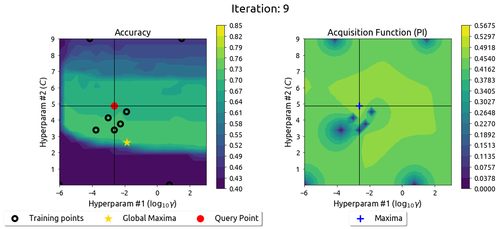
Above we see a slider showing the work of the Probability of Improvement acquisition function in finding the best hyperparameters.
上面我们看到一个滑块,显示改进概率采集函数在寻找最佳超参数方面的工作。

Above we see a slider showing the work of the Expected Improvement acquisition function in finding the best hyperparameters.
以上是一个滑块,显示了预期改进获取函数在寻找最佳超参数时的工作。
Comparison 对比
Below is a plot that compares the different acquisition functions. We ran the random acquisition function several times to average out its results.
下面是一个比较不同收获函数的图表。我们运行了随机收获函数多次以得出其结果的平均值。

All our acquisition beat the random acquisition function after seven iterations. We see the random method seemed to perform much better initially, but it could not reach the global optimum, whereas Bayesian Optimization was able to get fairly close. The initial subpar performance of Bayesian Optimization can be attributed to the initial exploration.
所有我们的获取在七次迭代之后都击败了随机获取函数。我们发现随机方法一开始似乎表现得更好,但它无法达到全局最优解,而贝叶斯优化能够得到相当接近。贝叶斯优化的最初表现不佳可以归因于最初的探索。
Other Examples 其他示例
Example 2 — Random Forest
示例 2 - 随机森林
Using Bayesian Optimization in a Random Forest Classifier.
在随机森林分类器中使用贝叶斯优化。
We will continue now to train a Random Forest on the moons dataset we had used previously to learn the Support Vector Machine model. The primary hyperparameters of Random Forests we would like to optimize our accuracy are the number of
Decision Trees we would like to have, the maximum depth for each of those decision trees.
我们将继续在之前用于训练支持向量机模型的"月亮"数据集上训练随机森林。我们希望优化随机森林的主要超参数以提高准确性,这些超参数包括我们想要的决策树数量和每棵决策树的最大深度。
The parameters of the Random Forest are the individual trained Decision Trees models.
随机森林的参数是各个经过训练的决策树模型。
We will be again using Gaussian Processes with Matern kernel to estimate and predict the accuracy function over the two hyperparameters.
我们将再次使用 Matern 核的高斯过程来估计和预测这两个超参数上的准确性函数。
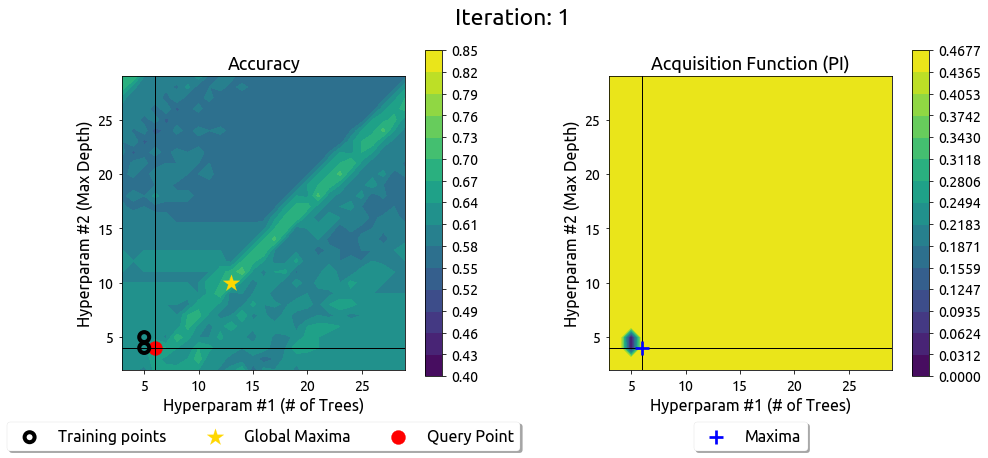
Above is a typical Bayesian Optimization run with the Probability of Improvement acquisition function.
以上是一个典型的贝叶斯优化运行,使用改进概率获取函数。

Above we see a run showing the work of the Expected Improvement acquisition function in optimizing the hyperparameters.
以上是一个运行示例,展示了期望改进获取函数在优化超参数方面的工作。
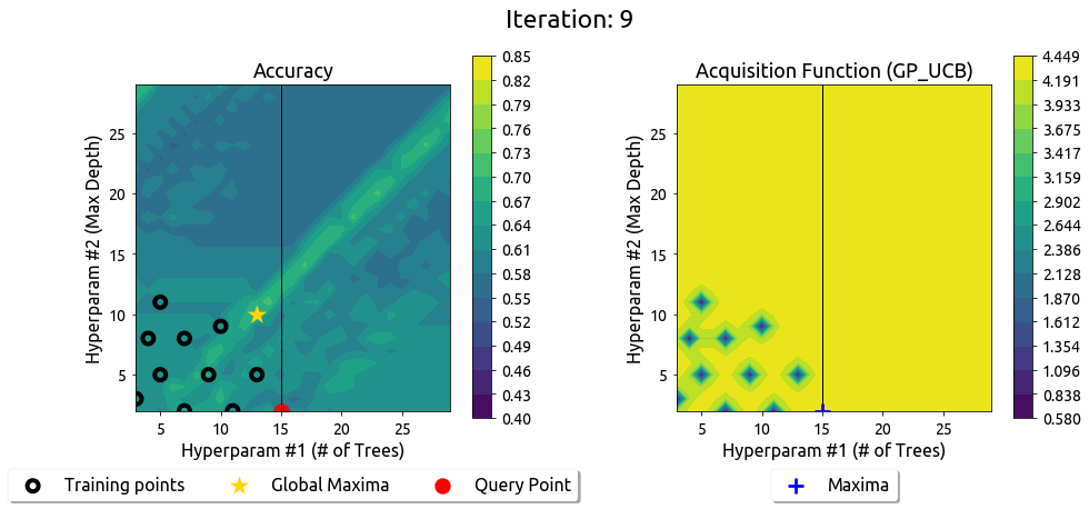
Now using the Gaussian Processes Upper Confidence Bound acquisition function in optimizing the hyperparameters.
现在在优化超参数时使用高斯过程上置信界限收获函数。
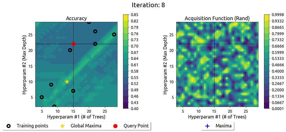
Let us now use the Random acquisition function.
让我们现在使用随机采集功能。

The optimization strategies seemed to struggle in this example. This can be attributed to the non-smooth ground truth. This shows that the effectiveness of Bayesian Optimization depends on the surrogate’s efficiency to model the actual black-box function. It is interesting to notice that the Bayesian Optimization framework still beats the random strategy using various acquisition functions.
在这个例子中,优化策略似乎遇到了困难。这可以归因于非光滑的真实数值。这表明,贝叶斯优化的有效性取决于替代模型对实际黑箱函数的模拟效率。有趣的是,贝叶斯优化框架仍然通过使用不同的获取函数击败了随机策略。
Example 3 — Neural Networks
示例 3 - 神经网络
Let us take this example to get an idea of how to apply Bayesian Optimization to train neural networks. Here we will be using scikit-optim, which also provides us support for optimizing function with a search space of categorical, integral, and real variables. We will not be plotting the ground truth here, as it is extremely costly to do so. Below are some code snippets that show the ease of using Bayesian Optimization packages for hyperparameter tuning.
让我们通过这个示例来了解如何应用贝叶斯优化来训练神经网络。在这里,我们将使用 scikit-optim ,它还为我们提供了对具有分类、整数和实数变量搜索空间的优化函数的支持。我们将不在这里绘制真实情况,因为这样做的成本非常昂贵。下面是一些代码片段,展示了使用贝叶斯优化软件包进行超参数调优的便利性。
The code initially declares a search space for the optimization problem. We limit the search space to be the following:
代码最初声明了优化问题的搜索空间。我们将搜索空间限制为以下内容:
-
batch_size — This hyperparameter sets the number of training examples to combine to find the gradients for a single step in gradient descent.
batch_size — 这个超参数设置了在梯度下降的单步中要组合的训练样本数量。
Our search space for the possible batch sizes consists of integer values s.t. batch_size = .
我们可能的批量大小搜索空间包括整数值,即 batch_size = 。 -
learning rate — This hyperparameter sets the stepsize with which we will perform gradient descent in the neural network.
学习率 — 该超参数设置了我们在神经网络中执行梯度下降的步长。
We will be searching over all the real numbers in the range .
我们将在范围 内搜索所有实数。 -
activation — We will have one categorical variable, i.e. the activation to apply to our neural network layers. This variable can take on values in the set .
激活 - 我们会有一个分类变量,即要应用于我们神经网络层的激活。这个变量可以取集合中的值 。
Now import gp-minimize 现在导入 gp-minimize scikit-optim.
注意:我们需要对准确度数值取反,因为我们正在使用 scikit-optim 中的最小化函数。scikit-optim to perform the optimization. Below we show calling the optimizer using Expected Improvement, but of course we can select from a number of other acquisition functions.
从 scikit-optim 导入以执行优化。下面我们展示如何使用期望改善来调用优化器,当然我们也可以从多种其他收益函数中进行选择。

In the graph above the y-axis denotes the best accuracy till then, and the x-axis denotes the evaluation number.
Looking at the above example, we can see that incorporating Bayesian Optimization is not difficult and can save a lot of time. Optimizing to get an accuracy of nearly one in around seven iterations is impressive!scikit-optim.
Let us get the numbers into perspective. If we had run this optimization using a grid search, it would have taken around iterations. Whereas Bayesian Optimization only took seven iterations. Each iteration took around fifteen minutes; this sets the time required for the grid search to complete around seventeen hours!
Conclusion and Summary 结论和摘要
In this article, we looked at Bayesian Optimization for optimizing a black-box function. Bayesian Optimization is well suited when the function evaluations are expensive, making grid or exhaustive search impractical. We looked at the key components of Bayesian Optimization. First, we looked at the notion of using a surrogate function (with a prior over the space of objective functions) to model our black-box function. Next, we looked at the “Bayes” in Bayesian Optimization — the function evaluations are used as data to obtain the surrogate posterior. We look at acquisition functions, which are functions of the surrogate posterior and are optimized sequentially. This new sequential optimization is in-expensive and thus of utility of us. We also looked at a few acquisition functions and showed how these different functions balance exploration and exploitation. Finally, we looked at some practical examples of Bayesian Optimization for optimizing hyper-parameters for machine learning models.
在本文中,我们研究了用于优化黑盒函数的贝叶斯优化。当函数评估昂贵时,贝叶斯优化非常适用,这使得网格或穷举搜索变得不切实际。我们研究了贝叶斯优化的关键组成部分。首先,我们考虑使用替代函数(带有对客体函数空间的先验)来对我们的黑盒函数进行建模。接下来,我们研究了“贝叶斯”中的贝叶斯优化——函数评估被用作数据来获得替代后验。我们研究了收获函数,这些函数是替代后验的函数,并且是依次优化的。这种新的顺序优化成本低廉,因此对我们是有用的。我们还研究了一些收获函数,并展示了这些不同函数如何平衡探索和开发。最后,我们研究了一些关于用于优化机器学习模型的贝叶斯优化的实际示例。
We hope you had a good time reading the article and hope you are ready to exploit the power of Bayesian Optimization. In case you wish to explore more, please read the Further Reading section below. We also provide our repository to reproduce the entire article.
我们希望您阅读本文时过得愉快,并且希望您准备利用贝叶斯优化的力量。如果您希望了解更多信息,请阅读下面的进一步阅读部分。我们还提供我们的存储库以重新现整篇文章。