解锁专家、大师和宗师天才级别的更复杂操作符。
Arithmetic 算术
add(x, y, 过滤 = false), x + y
添加所有输入(至少需要 2 个输入)。如果 filter = true,则在添加之前将所有输入的 NaN 过滤为 0
将许多桶的分组字段转换为仅有的少量可用桶,以便使处理分组字段在计算上更高效
This operator converts a grouping field with many buckets into a lesser number of only the available buckets, making working with grouping fields computationally efficient. The example below will clarify the implementation.
此操作将具有许多桶的分组字段转换为仅包含可用桶的较少数量,使分组字段的处理在计算上更高效。以下示例将阐明实现方式。
Example: 示例:
Say a grouping field is provided as an integer (e.g., industry: tech -> 0, airspace -> 1, ...) and for a certain date, we have instruments with grouping field values among {0, 1, 2, 99}. Instead of creating 100 buckets and keeping 96 of them empty, it is better to just create 4 buckets with values {0, 1, 2, 3}. So, if the number of unique values in x is n, densify maps those values between 0 and (n-1). The order of magnitude need not be preserved.
一个分组字段以整数形式提供(例如,行业:技术 -> 0,空域 -> 1,...),对于某个日期,我们有分组字段值在{0,1,2,99}之间的仪器。与其创建 100 个桶并保留其中的 96 个为空,不如只创建 4 个桶,其值为{0,1,2,3}。因此,如果 x 中唯一值的数量为 n,则将这些值映射到 0 和(n-1)之间。不需要保留数量级。
除以(x, y), x / y
自然对数。例如:Log(高/低)使用高/低比的自然对数作为股票权重。
所有输入的最大值。至少需要 2 个输入
Example: 示例:
Simulation Settings 模拟设置
| Region 区域 | Universe 宇宙 | Language 语言 | Decay 衰减 | Delay 延迟 | Truncation 截断 | Neutralization 中和 | Pasteurization 巴氏杀菌 | NaN Handling 处理 NaN | Unit Handling 单元处理 |
|---|---|---|---|---|---|---|---|---|---|
| USA | TOP3000 | Fast Expression 快速表达式 | 2 | 1 | 0.01 | Industry 行业 | On 在 | Off 关闭 | Verify 验证 |
所有输入的最小值。至少需要 2 个输入
Example: 示例:
Simulation Settings 模拟设置
| Region 区域 | Universe 宇宙 | Language 语言 | Decay 衰减 | Delay 延迟 | Truncation 截断 | Neutralization 中和 | Pasteurization 巴氏杀菌 | NaN Handling 处理 NaN | Unit Handling 单元处理 |
|---|---|---|---|---|---|---|---|---|---|
| USA | TOP3000 | Fast Expression 快速表达式 | 3 | 1 | 0.01 | Industry 行业 | On 在 | Off 关闭 | Verify 验证 |
乘以(x, y, ..., 过滤器=false), x * y
将所有输入相乘。至少需要 2 个输入。将 NaN 值设置为 1
Examples: 示例:
Simulation Settings 模拟设置
| Region 区域 | Universe 宇宙 | Language 语言 | Decay 衰减 | Delay 延迟 | Truncation 截断 | Neutralization 中和 | Pasteurization 巴氏杀菌 | NaN Handling 处理 NaN | Unit Handling 单元处理 |
|---|---|---|---|---|---|---|---|---|---|
| USA | TOP3000 | Fast Expression 快速表达式 | 3 | 1 | 0.01 | Industry 行业 | On 在 | Off 关闭 | Verify 验证 |
如果输入为 NaN;则返回 NaN
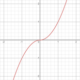
x 的 y 次幂,使得最终结果保留 x 的符号
sign(x) * (abs(x) ^ y)
sign(x) * (|x| ^ y)
x raised to the power of y such that final result preserves sign of x. For power of 2, x ^ y will be a parabola but signed_power(x, y) will be odd and one-to-one function (unique value of x for certain value of signed_power(x, y)) unlike parabola.
x 的 y 次幂,使得最终结果保留 x 的符号。对于 2 的幂,x^y 将是一个抛物线,但 signed_power(x, y)将是奇函数且一一对应(对于 signed_power(x, y)的特定值,x 的唯一值)与抛物线不同。
Example: 示例:
If x = 3, y = 2 ⇒ abs(x) = 3 ⇒ abs(x) ^ y = 9 and sign(x) = +1 ⇒ sign(x) * (abs(x) ^ y) = signed_power(x, y) = 9
如果 x = 3,y = 2 ⇒ abs(x) = 3 ⇒ abs(x) ^ y = 9 并且 sign(x) = +1 ⇒ sign(x) * (abs(x) ^ y) = signed_power(x, y) = 9
If x = -9, y = 0.5 ⇒ abs(x) = 9 ⇒ abs(x) ^ y = 3 and sign(x) = -1 ⇒ sign(x) * (abs(x) ^ y) = signed_power(x, y)
如果 x = -9,y = 0.5 则 abs(x) = 9 则 abs(x) ^ y = 3 且 sign(x) = -1 则 sign(x) * (abs(x) ^ y) = signed_power(x, y)
减去(x, y, 过滤器=false), x - y
x-y。如果 filter = true,在减法之前将所有输入的 NaN 过滤为 0
Logical 逻辑
逻辑与运算符,当两个操作数都为真时返回 true,否则返回 false
if_else(输入 1, 输入 2, 输入 3)
如果 input1 为真则返回 input2 否则返回 input3。
if_else(event_condition, Alpha_expression_1, Alpha_expression_2)
if_else(事件条件, 表达式 1, 表达式 2)
If the event condition provided is true, Alpha_expression_1 will be returned. If the event condition provided is false, Alpha_expression_2 will be returned.
如果提供的事件条件为真,将返回 Alpha_expression_1。如果提供的事件条件为假,将返回 Alpha_expression_2。
Example: 示例:
We are interested in testing our hypothesis that if the stock price of a company has increased over the last 2 days, it may decrease in the future. Also, if the number of stocks bought and sold today is higher than the monthly average, then the reversion effect may be observed more profoundly.
我们对测试以下假设感兴趣:如果一家公司的股价在过去两天内上涨,那么它未来可能会下跌。此外,如果今天买卖的股票数量高于月均水平,那么回归效应可能会更加明显。
We will implement this hypothesis by taking positions according to the difference of close price today and 3 days ago with alpha_2 using the ts_delta operator. When current volume is higher than average daily volume, we will take a larger position by multiplying by 2 to get alpha_1.
我们将通过使用 ts_delta 操作符,根据今天收盘价与三天前收盘价的差异,利用 alpha_2 来采取立场。当当前成交量高于平均每日成交量时,我们将通过乘以 2 来采取更大的立场,以获得 alpha_1。
Simulation Settings 模拟设置
| Region 区域 | Universe 宇宙 | Language 语言 | Decay 衰减 | Delay 延迟 | Truncation 截断 | Neutralization 中和 | Pasteurization 巴氏杀菌 | NaN Handling 处理 NaN | Unit Handling 单元处理 |
|---|---|---|---|---|---|---|---|---|---|
| USA | TOP3000 | Fast Expression 快速表达式 | 3 | 1 | 0.01 | Industry 行业 | On 在 | Off 关闭 | Verify 验证 |
如果 input1 小于 input2 则返回 true,否则返回 false
返回 true 如果 input1 <= input2,否则返回 false
返回 true 如果两个输入相同,否则返回 false
逻辑比较运算符用于比较两个输入
返回值为 true,如果 input1 大于等于 input2,否则返回 false
返回 true 如果两个输入不相同,否则返回 false
如果(输入 == NaN)则返回 1 否则返回 0
返回 x 的逻辑否定。如果 x 为真(1),则返回假(0),如果输入为假(0),则返回真(1)。
逻辑或运算符在任一或两个输入为真时返回真,否则返回假
Time Series 时间序列
自上次 x 变更以来的天数
限制输入变化的数量和幅度(从而减少周转)
hump(x, hump = 0.01) hump(x, hump=0.01)
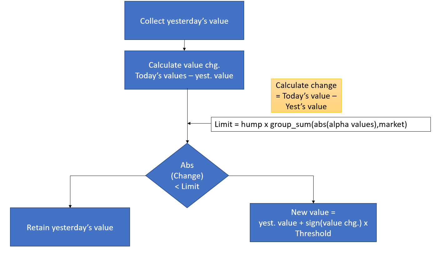
This operator limits the frequency and magnitude of changes in the Alpha (thus reducing turnover). If today's values show only a minor change (not exceeding the Threshold) from yesterday's value, the output of the hump operator stays the same as yesterday. If the change is bigger than the limit, the output is yesterday's value plus the limit in the direction of the change.
此操作员限制 Alpha(因此减少周转率)的变化频率和幅度。如果今天的值仅显示与昨天值相比的微小变化(不超过阈值),则驼峰操作员的输出与昨天相同。如果变化超过限制,则输出为昨天的值加上变化方向上的限制。
This operator may help reduce turnover and drawdown.
此操作员可能有助于降低周转率和赎回率。
Flowchart of the Hump operator:
流程图中的驼峰运算符:
Simulation Settings 模拟设置
| Region 区域 | Universe 宇宙 | Language 语言 | Decay 衰减 | Delay 延迟 | Truncation 截断 | Neutralization 中和 | Pasteurization 巴氏杀菌 | NaN Handling 处理 NaN | Unit Handling 单元处理 |
|---|---|---|---|---|---|---|---|---|---|
| USA | TOP3000 | Fast Expression 快速表达式 | 3 | 1 | 5 | Market 市场 | On 在 | Off 关闭 | Verify 验证 |
返回通过查看回望日数得到的第 K 个输入值。此操作符可以在 k=1 时用于回补缺失数据。
Returns k-th value of input by looking through lookback days while ignoring space separated scalars in ignore list. This operator is also known as backfill operator as it can be used to backfill missing data.
通过查看回望日数来返回输入的第 k 个值,同时忽略忽略列表中以空格分隔的标量。此操作符也称为回填操作符,因为它可以用来回填缺失的数据。
ignore parameter is used to provide list of separated scalars to ignore from counting
忽略参数用于提供要忽略计数的分隔标量列表
Example of backfill: 回填示例:
Simulation Settings 模拟设置
| Region 区域 | Universe 宇宙 | Language 语言 | Decay 衰减 | Delay 延迟 | Truncation 截断 | Neutralization 中和 | Pasteurization 巴氏杀菌 | NaN Handling 处理 NaN | Unit Handling 单元处理 |
|---|---|---|---|---|---|---|---|---|---|
| USA | TOP3000 | Fast Expression 快速表达式 | 3 | 1 | 0.01 | Industry 行业 | On 在 | Off 关闭 | Verify 验证 |
返回过去 d 天内与当前 x 值不相同的最后 x 个值
返回过去 d 天内时间序列中最大值的相对索引。如果当前天是过去 d 天内的最大值,则返回 0。如果前一天是过去 d 天内的最大值,则返回 1。
It returns the relative index of the max value in the time series for the past d days. If the current day has the max value for the past d days, it returns 0. If previous day has the max value for the past d days, it returns 1.
返回过去 d 天内时间序列中最大值的相对索引。如果当前天是过去 d 天内的最大值,则返回 0。如果前一天是过去 d 天内的最大值,则返回 1。
Example: 示例:
If d = 6 and values for past 6 days are [6,2,8,5,9,4] with first element being today’s value then max value is 9 and it is present 4 days before today. Hence, ts_arg_max(x, d) = 4
如果 d = 6 且过去 6 天的值为 [6,2,8,5,9,4],其中第一个元素是今天的值,则最大值为 9,它出现在今天之前 4 天。因此,ts_arg_max(x, d) = 4
返回过去 d 天内时间序列中最小值的相对索引;如果当前天是过去 d 天内的最小值,则返回 0;如果前一天是过去 d 天内的最小值,则返回 1。
ts_arg_min(x, d)
It returns the relative index of the min value in the time series for the past d days. If the current day has the min value for the past d days, it returns 0. If previous day has the min value for the past d days, it returns 1.
返回过去 d 天内时间序列中最小值的相对索引。如果当前天是过去 d 天内的最小值,则返回 0。如果前一天是过去 d 天内的最小值,则返回 1。
Example: 示例:
If d = 6 and values for past 6 days are [6,2,8,5,9,4] with first element being today’s value then min value is 2 and it is present 4 days before today. Hence, ts_arg_min(x, d) = 1
如果 d = 6 且过去 6 天的值为 [6,2,8,5,9,4],其中第一个元素是今天的值,则最小值为 2,它出现在今天之前 4 天。因此,ts_arg_min(x, d) = 1
返回 x - tsmean(x, d),但会小心处理 NaN。也就是说,在计算平均值时忽略 NaN。
This operator returns x – ts_mean(x, d), but it deals with NaNs carefully
此操作符返回 x – ts_mean(x, d),但它会小心处理 NaN 值
Example: 示例:
If d = 6 and values for past 6 days are [6,2,8,5,9,NaN] then ts_mean(x,d) = 6 since NaN are ignored from mean computation. Hence, ts_av_diff(x,d) = 6-6 = 0
如果 d = 6 且过去 6 天的值为 [6,2,8,5,9,NaN],则 ts_mean(x,d) = 6,因为 NaN 在计算平均值时被忽略。因此,ts_av_diff(x,d) = 6-6 = 0
ts_backfill(x, lookback = d, k=1, ignore="NAN")
回填是将 NAN 或 0 值替换为有意义的值(即第一个非 NAN 值)的过程
ts_backfill(x,lookback = d, k=1, ignore="NAN")
ts_backfill(x, lookback = d, k=1, ignore="NAN")
The ts_backfill operator replaces NaN values with the last available non-NaN value. If the input value of the data field x is NaN, the ts_backfill operator will check available input values of the same data field for the past d number of days, and output the most recent available non-NaN input value. If the k parameter is set, then the ts_backfill operator will output the kth most recent available non-NaN input value.
ts_backfill 运算符将 NaN 值替换为最后一个可用的非 NaN 值。如果数据字段 x 的输入值为 NaN,ts_backfill 运算符将检查过去 d 天内的相同数据字段的可用输入值,并输出最近的可用的非 NaN 输入值。如果设置了 k 参数,则 ts_backfill 运算符将输出第 k 个最近的可用的非 NaN 输入值。
This operator improves weight coverage and may help to reduce drawdown risk.
此操作员提高权重覆盖率,可能有助于降低回撤风险。
Example: ts_backfill(x, 252)
示例:ts_backfill(x, 252)
- If the input value for data field x = non-NaN, then output = x
如果数据字段 x 的输入值非 NaN,则输出=x - If the input value for data field x = NaN, then output = most recent available non-NaN input value for x in the past 252 days
如果数据字段 x 的输入值为 NaN,则输出=过去 252 天内 x 的最新可用非 NaN 输入值
返回过去 d 天的 x 和 y 的相关性
ts_corr(x, y, d)
Pearson correlation measures the linear relationship between two variables. It's most effective when the variables are normally distributed and the relationship is linear.
皮尔逊相关系数衡量两个变量之间的线性关系。当变量呈正态分布且关系为线性时,其效果最为显著。
Example:
Simulation Settings
| Region | Universe | Language | Decay | Delay | Truncation | Neutralization | Pasteurization | NaN Handling | Unit Handling |
|---|---|---|---|---|---|---|---|---|---|
| USA | TOP3000 | Fast Expression | 3 | 1 | 0.01 | Industry | On | Off | Verify |
ts_decay_linear(x, d, dense = false)
Returns the linear decay on x for the past d days. Dense parameter=false means operator works in sparse mode and we treat NaN as 0. In dense mode we do not. Data smoothing techniques like linear decay reduce noise in time-series data by applying a decay factor to older observations, which helps to stabilize the dataset.
This operator improves turnover and drawdown.
Example:
- For a stock with the following prices over the last 5 days:
- Day 0: 30 (outlier)
- Day -1: 5
- Day -2: 4
- Day -3: 5
- Day -4: 6
- The calculation would be:
- Numerator = (30⋅5)+(5⋅4)+(4⋅3)+(5⋅2)+(6⋅1)=150+20+12+10+6=198
- Denominator=5+4+3+2+1=15
- Weighted Average=198/15=13.2
- The weighted average value of 13.2 is used instead of the outlier value of 20 for assigning weight.
ts_regression(y, x, d, lag = 0, rettype = 0)
Given a set of two variables’ values (X: the independent variable, Y: the dependent variable) over a course of d days, an approximating linear function can be defined, such that sum of squared errors on this set assumes minimal value:
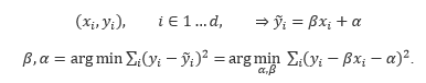
Beta and Alpha in second line are OLS Linear Regression coefficients.
ts_regression operator returns various parameters related to said regression. This is governed by “rettype” keyword argument, which has a default value of 0. Other “rettype” argument values correspond to:

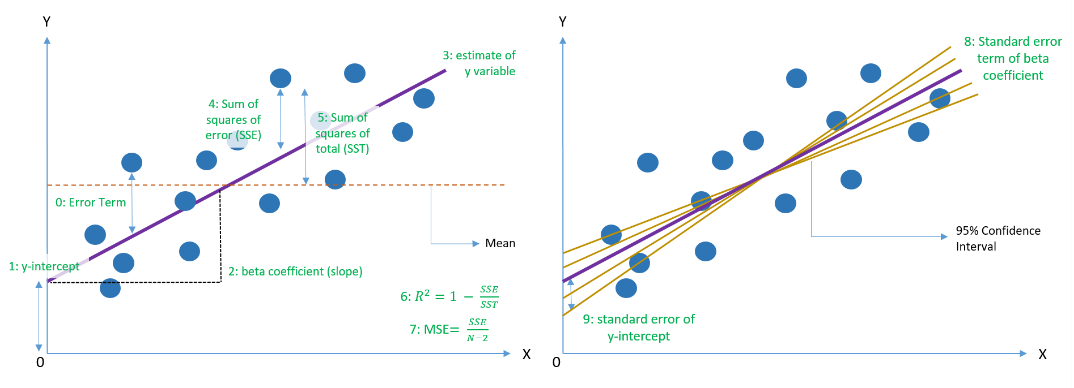
Here, "di" is current day index, “n”(may differ from d) is a number of valid (x, y) tuples used for calculation. All summations are over day index, using only valid tuples.
“lag” keyword argument may be optionally specified (default value is zero) to calculate lagged regression parameters instead:
Example:
- ts_regression(est_netprofit, est_netdebt, 252, lag = 0, rettype = 2)
- Taking the data from the past 252 trading days (1 year), return the β coefficient from the equation when estimating the est_netprofit using the est_netdebt
- ts_regression(est_netprofit, est_netdebt, 252, lag = 0, rettype = 2)
Simulation Settings
| Region | Universe | Language | Decay | Delay | Truncation | Neutralization | Pasteurization | NaN Handling | Unit Handling |
|---|---|---|---|---|---|---|---|---|---|
| USA | TOP3000 | Fast Expression | 3 | 1 | 5 | Market | On | Off | Verify |
This operator returns (x – ts_min(x, d)) / (ts_max(x, d) – ts_min(x, d)) + constant
This operator is similar to scale down operator but acts in time series space
Example:
If d = 6 and values for last 6 days are [6,2,8,5,9,4] with first element being today’s value, ts_min(x,d) = 2, ts_max(x,d) = 9
ts_scale(x,d,constant = 1) = 1 + (6-2)/(9-2) = 1.57
Cross Sectional
normalize(x, useStd = false, limit = 0.0)
This operator calculates the mean value of all valid alpha values for a certain date, then subtracts that mean from each element. If useStd= true, the operator calculates the standard deviation of the resulting values and divides each normalized element by it. If limit is not equal to 0.0, operator puts the limit of the resulting alpha values (between -limit to + limit).
Example:
If for a certain date, instrument value of certain input x is [3,5,6,2], mean = 4 and standard deviation = 1.82
normalize(x, useStd = false, limit = 0.0) = [3-4,5-4,6-4,2-4] = [-1,1,2,-2]
normalize(x, useStd = true, limit = 0.0) = [-1/1.82,1/1.82,2/1.82,-2/1.82] = [-0.55,0.55,1.1,-1.1]
quantile(x, driver = gaussian, sigma = 1.0)
Rank the input raw Alpha vector
The ranked Alpha value would be within [0, 1]
- Shift the ranked Alpha vector
For every Alpha value in the ranked Alpha vector, it is shifted as: Alpha_value = 1/N + Alpha_value * (1 - 2/N), here assume there are N instruments with value in the Alpha vector. The shifted Alpha value would be within [1/N, 1-1/N] - Apply distribution for each Alpha value in the ranked Alpha vector using the specified driver. Driver can be one of "gaussian", "uniform", "cauchy".
Note : Sigma only affects the scale of the final value.
This operator may help reduce outliers.
Example:
Simulation Settings
| Region | Universe | Language | Decay | Delay | Truncation | Neutralization | Pasteurization | NaN Handling | Unit Handling |
|---|---|---|---|---|---|---|---|---|---|
| USA | TOP3000 | Fast Expression | 3 | 1 | 0.01 | Market | On | Off | Verify |
rank(x, rate=2):
The Rank operator ranks the value of the input data x for the given stock among all instruments, and returns float numbers equally distributed between 0.0 and 1.0. When rate is set to 0, the sorting is done precisely. The default value of rate is 2.
This operator may help reduce outliers and drawdown while improving the Sharpe.
Example:
Rank(close); Rank (close, rate=0) # Sorts precisely
X = (4,3,6,10,2) => Rank(x) = (0.5, 0.25, 0.75, 1, 0)
scale (x, scale=1, longscale=1, shortscale=1)
The operator scales the input to the book size. We can optionally tune the book size by specifying the additional parameter 'scale=booksize_value'. We can also scale the long positions and short positions to separate scales by specifying additional parameters: longscale=long_booksize and shortscale=short_booksize. The default value of each leg of the scale is 0, which means no scaling, unless specified otherwise. Scale the alpha so that the sum of abs(x) over all instruments equals 1. To scale to a different book size, use Scale(x) * booksize.
This operator may help reduce outliers.
Please check examples for the application of the same
Examples:
scale(returns, scale=4); scale (returns, scale= 1) + scale (close, scale=20); scale (returns, longscale=4, shortscale=3)
zscore(x)
Z-score is a statistical tool that indicates how many standard deviations a data point lies from the average of a group of values. Essentially, it measures how unusual a data point is in relation to the mean, making it a handy tool for understanding deviation and comparison.
The formula to calculate a Z-score is:
Where:
- x is an individual data point
- mean(x) is the average of the data set
- std(x) is the standard deviation of the data set
By this definition, the mean of the Z-scores in a distribution is always 0, and the standard deviation is always 1.
A Z-score tells you how many standard deviations a particular data point is from the mean. If the Z-score is positive, the data point is above the mean, and if it's negative, it's below the mean.
Z-scores may be especially useful for normalizing and comparing different data fields for different stocks or different data fields. They allow researchers to calculate the probability of a score occurring within a standard normal distribution and compare two scores that are from different samples (which may have different means and standard deviations).
This operator may help reduce outliers.
Simulation Settings
| Region | Universe | Language | Decay | Delay | Truncation | Neutralization | Pasteurization | NaN Handling | Unit Handling |
|---|---|---|---|---|---|---|---|---|---|
| USA | TOP3000 | Fast Expression | 3 | 1 | 0.03 | Market | On | Off | Verify |
Vector
Transformational
Bucket
Convert float values into indexes for user-specified buckets. Bucket is useful for creating group values, which can be passed to group operators as input.
If buckets are specified as "num_1, num_2, …, num_N", it is converted into brackets consisting of [(num_1, num_2, idx_1), (num_2, num_3, idx_2), ..., (num_N-1, num_N, idx_N-1)]
Thus with buckets="2, 5, 6, 7, 10", the vector "-1, 3, 6, 8, 12" becomes "0, 1, 2, 4, 5"
If range if specified as "start, end, step", it is converted into brackets consisting of [(start, start+step, idx_1), (start+step, start+2*step, idx_2), ..., (start+N*step, end, idx_N)].
Thus with range="0.1, 1, 0.1", the vector "0.05, 0.5, 0.9" becomes "0, 4, 8"
Note that two hidden buckets corresponding to (-inf, start] and [end, +inf) are added by default. Use the skipBegin, skipEnd parameters to remove these buckets. Use skipBoth to set both skipEnd and skipBegin to true.
If you want to assign all NAN values into a separate group of their own, use NANGroup. The index value will be one after the last bucket
Examples:
my_group = bucket(rank(volume), range="0.1,1,0.1");
group_neutralize(sales/assets, my_group)
my_group = bucket(rank(volume), buckets ="0.2,0.5,0.7", skipBoth=True, NANGroup=True);
group_neutralize(sales/assets, my_group)
This operator can be used to change Alpha values only under a specified condition and to retain Alpha values in other cases. It also allows for closing Alpha positions (assigning NaN values) under a specified condition.
Trade_When (x=triggerTradeExp, y=AlphaExp, z=triggerExitExp)
If triggerExitExp > 0, Alpha = NaN.
Else if triggerTradeExp > 0, Alpha = AlphaExp;
else, Alpha = previousAlpha
This operator may help reduce correlation and reduce turnover.
Examples:
Trade_When (volume >= ts_sum(volume,5)/5, rank(-returns), -1)
If (volume >= ts_sum(volume,5)/5), Alpha = rank(-returns);
else trade previous Alpha;
exit condition is always false.
Trade_When (volume >= ts_sum(volume,5)/5, rank(-returns), abs(returns) > 0.1)
If abs(returns) > 0.1, Alpha = nan;
else if volume >= ts_sum(volume,5)/5, Alpha = rank(-returns);
else trade previous Alpha.
Group
group_backfill(x, group, d, std = 4.0)
If a certain value for a certain date and instrument is NaN, from the set of same group instruments, calculate winsorized mean of all non-NaN values over last d days. Winsorized mean means inputs are truncated by std * stddev where stddev is the standard deviation of inputs.
Example:
If d = 4 and there are 3 instruments(i1, i2, i3) in a group whose values for past 4 days are x[i1] = [4,2,5,5], x[i2] = [7,NaN,2,9], x[i3] = [NaN,-4,2,NaN] where first element is most recent, then if we want to backfill x, we will only have to backfill x[i3]’s first element because every other instrument’s first element is non-NaN.
The non-NaN values of other groups are [4,2,5,5,7,2,9,-4,2]. Mean = 3.56, Standard deviation is 3.71 and none of the item is outside the range of 3.56 – 4 * 3.71 and 3.56 + 4 * 3.71. Hence, we don’t need to clip elements to those limits. Hence, Winsorized mean = backfilled value = 3.56.
For three instruments, group_backfill(x, group, d, std = 4.0) = [4,7,3.56]
group_neutralize(x, group)
Neutralize alpha against groups. Difference between normalize and group_neutralize is in normalize, every element is subtracted by mean of all values of all instruments on that day whereas in group_neutralize, element is subtracted by mean of all values of the group of instruments that it belongs on that day.
This operator may help reduce correlation, depending on the neutralization used.
Example:
If values of field x on a certain date for 10 instruments is [3,2,6,5,8,9,1,4,8,0] and first 5 instruments belong to one group, last 5 belong to other, then mean of first group = (3+2+6+5+8)/5 = 4.8 and mean of second group = (9+1+4+8+0)/5 = 4.4. Subtracting means from instruments of respective groups gives [3-4.8, 2-4.8, 6-4.8, 5-4.8, 8-4.8, 9-4.4, 1-4.4, 4-4.4, 8-4.4, 0-4.4] = [-1.8, -2.8, 1.2, 0.2, 3.2, 4.6, -3.4, -0.4, 3.6, -4.4]
group_rank(x, group)
Group operators are a type of cross-sectional operator that compares stocks at a finer level, where the cross-sectional operation is applied within each group, rather than across the entire market. The group_rank operator allocates the stocks to their specified group, then within each group, it ranks the stocks based on their input value for data field x and returns an equally distributed number between 0.0 and 1.0.
This operator may help reduce both outliers and drawdown while reducing correlation.
Example: group_rank(x, subindustry)
- The stocks are first grouped into their respective subindustry.
- Within each subindustry, the stocks within that subindustry are ranked based on their input value for data field x and assigned an equally distributed number between 0.0 and 1.0.