Research on Measurement Method of Leaf Length and Width Based on Point Cloud

Abstract

Leaf is an important organ for photosynthesis and transpiration associated with the plants’ growth. Through the study of leaf phenotype, it the physiological characteristics produced by the interaction of the morphological parameters with the environment can be understood. In order to realize the assessment of the spatial morphology of leaves, a method based on three-dimensional stereo vision was introduced to extract the shape information, including the length and width of the leaves. Firstly, a depth sensor was used to collect the point cloud of plant leaves. Then, the leaf coordinate system was adjusted by principal component analysis to extract the region of interest; and compared with a cross-sectional method, the geodesic distance method, we proposed a method based on the cutting plane to obtain the intersecting line of the three-dimensional leaf model. Eggplant leaves were used to compare the accuracy of these methods in the measurement of a single leaf.
叶子是植物生长中与光合作用和蒸腾作用相关的重要器官。通过研究叶片表型，可以理解由形态参数与环境相互作用产生的生理特征。为了实现叶片空间形态的评估，引入了一种基于三维立体视觉的方法来提取形状信息，包括叶片的长度和宽度。首先，使用深度传感器收集植物叶片的点云。然后，通过主成分分析调整叶片坐标系以提取感兴趣区域；并与横截面法、测地线距离法相比，我们提出了一种基于切割平面的方法来获得三维叶片模型的交线。使用茄子叶片来比较这些方法在单叶测量中的准确性。

1. Introduction

Leaf is the main organ of plants for photosynthesis and transpiration, and plant growth information is closely related to leaf parameters. Mastering the growth rule of plant leaves is of guiding significance for cultivation. Plant growth information is closely related to leaf parameters, which is of great significance for high efficiency and yield. Leaf parameters have a profound impact on activities such as plant growth and development, so scientifically determining leaf parameters is of great significance [1]. Leaf shape parameters such as leaf area, thickness, length, width, and leaf shape index are important indicators for evaluating the impact of plant environmental factors. With the rapid development of science and technology, automatic measurement technology has been widely used in life, as well as agriculture [2]. Compared with the manual measurement of leaf parameter measurement technology, automatic measurement has the advantages of fast speed, high precision and real-time performance, which greatly improves the efficiency of leaf parameters measurement.

Currently, leaf length and width are important shape parameters, which can be used in tasks such as leaf area estimation and automatic recognition. High-performance technology has been used to measure the linear distance between leaf petiole and tip [3,4,5,6], the shortest distance between leaf petiole and tip [7,8], or extraction skeleton between the petiole and tip [9,10]. Grid and scanning methods are commonly used for leaf measurement, which are simple to implement, but require some manpower and time [11]. The scanner method is to image plant leaves [12], and then use Photoshop, ArcGIS or other softwares to count the pixels and determine the leaf information of the plant. Measurement based on image processing has the advantages of simple and fast operation [13,14,15]. For leaf measurement, the common method is to extract the minimum enclosing rectangle [16,17]. The minimum enclosing rectangles and the aspect rations of leaves were obtained by Hotelling transform [18] or rotation matrix [19]. For improvement of the minimum bounding box, Xiang et al. [20] rotated and moved main axis of leaf image, compared the size of the area surrounded by the boundary. Guo et al. [21] applied poly-line fitting to detect the media axis, and fitting the length of the line as the leaf length measurement.

With the rapid development of 3D technology, the research of three-dimensional measurement technology has been applied to the automatic reconstruction of animal body size, such as pig [22,23], sheep [24], and cattle [25]. The measurement of human body size plays an important role and 3D scanning technology has been used to automatically measure body size in a non-contact way [26], for example, Liu et al. [27] and Tan et al. [28] obtained the size of a human body via random forest regression analysis of geodesic distances to extract the feature points and lines. Zhang et al. [29] proposed a framework for pose estimation from range images by geodesic distance. 3D technology is also used in earthwork [30], water conservancy [31] and other complex terrain problems, to achieve the reconstruction and measurement. In the current study, image analysis was used to quantify crop characteristics, which are critical for the marketability of new varieties [32,33]. Zhou et al. [34] obtained three-dimensional structural data of lodged maize using an unmanned aerial vehicle. Guo [35], Gongal [36] and Yang et al. [37] reconstructed apple tree canopy and extracted the apple diameter based on a 3D camera. Using a 3D point cloud to measure plant leaf information has become an emerging area of scientific research. In plant growth monitoring, accurate and nondestructive measurement of plant structure parameters is very important, Zhang et al. [38] developed a multi-camera photography system and measured six variables of 3D nursery paprika plants’ models. Feng et al. [39] based on photometric stereo vision determined the normal vectors’ distribution and fitted the leaf’s space plane. Zhang et al. [40] scanned the plant vertically with the laser sheet and obtained point cloud structure of the sample. Itakura et al. [41] segmented leaves in the top-view images by distance transform and expanded the seed region by watershed algorithm with the 3D information. Hu et al. [42] proposed a 3D point cloud filtering method for leaves based on manifold distance and normal estimation and pointed out that the distance between two points cannot reflect all of the manifold similarities well, while the geodesic curve better reflects the similarities between these two points. It can be seen that the cross-sectional method and geodesic distance are the most commonly used methods in 3D length measurement. Leaf is a research object with spatial attributes, so we compare the cross-section method and geodesic distance method to measure the length and width of leaf on three-dimensional model. The method is improved on the basis of the cross-section method, so that it can quickly obtain the intersection line.
随着 3D 技术的快速发展，三维测量技术的研究已应用于动物体型的自动重建，如猪[22, 23]、羊[24]和牛[25]。人体尺寸的测量发挥着重要作用，3D 扫描技术已被用于非接触式自动测量人体尺寸[26]，例如，刘等[27]和谭等[28]通过地理距离的随机森林回归分析提取特征点和线，获得了人体尺寸。张等[29]提出了一种基于测地距离的姿态估计框架。3D 技术还应用于土方工程[30]、水利[31]和其他复杂地形问题，以实现重建和测量。在当前研究中，图像分析被用于量化作物特征，这对于新品种的市场化至关重要[32, 33]。周等[34]使用无人机获得了倒伏玉米的三维结构数据。郭[35]、贡加尔[36]和杨等。 [ 37] 重建苹果树树冠并基于 3D 相机提取苹果直径。使用 3D 点云测量植物叶片信息已成为科学研究的崭新领域。在植物生长监测中，准确且非破坏性的测量植物结构参数非常重要，张等[ 38]开发了一种多摄像头摄影系统，并测量了 3D 苗圃辣椒植物模型的六个变量。冯等[ 39]基于光度立体视觉确定了法向量的分布并拟合了叶片的空间平面。张等[ 40]用激光片垂直扫描植物并获得了样品的点云结构。板仓等[ 41]通过距离变换在俯视图图像中分割叶片，并利用 3D 信息通过流域算法扩展种子区域。胡等[ 42]提出了一种基于流形距离和法向估计的叶片 3D 点云滤波方法，并指出两点之间的距离不能很好地反映所有流形相似性，而测地线曲线更好地反映了这两点之间的相似性。 可以看出，横断面法和大地测量距离法是三维长度测量中最常用的方法。叶片是一个具有空间属性的科研对象，因此我们比较横断面法和大地测量距离法来测量叶片在三维模型上的长度和宽度。该方法在横断面法的基础上进行了改进，以便快速获得交线。

2. Materials and Methods

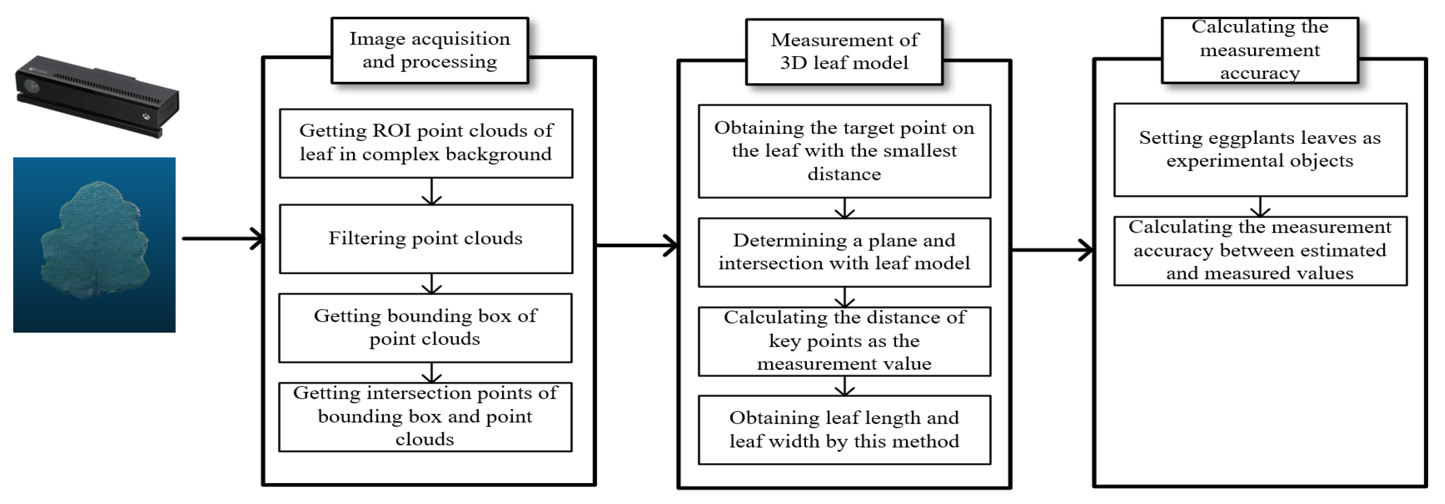
2.1. Acquisition the RoI of Leaf Point Cloud Model

Kinect2.0 was used to photograph eggplant and get the corresponding point cloud to obtain complete scene information. The scene information contains the entire plant, and the research object is the length and width of a leaf, so a complete leaf point cloud without occlusion was manually selected as the experimental object. The length measurement did not include the length of the petiole, so the petiole was removed manually to ensure the accuracy of measurement. Here, eggplant leaves were selected as the research object to prove the effectiveness of the measurement of leaf length and width. The extracted leaf point cloud information contained noise, so the filtering method [43] and smoothing algorithm [44] provided by Point Cloud Library were used to process the point cloud in Figure 1.
Kinect2.0 用于拍摄茄子并获取相应的点云以获取完整的场景信息。场景信息包含整个植物，研究对象是叶片的长度和宽度，因此手动选取了无遮挡的完整叶片点云作为实验对象。长度测量不包括叶柄长度，因此手动移除了叶柄以确保测量的准确性。在此，选择茄子叶片作为研究对象以证明测量叶片长度和宽度的有效性。提取的叶片点云信息包含噪声，因此使用了点云库提供的[43]滤波方法和[44]平滑算法对图 1 中的点云进行处理。

Figure 1. Operation flowchart of the system.

When collecting data, the distance between kinect2.0 and the shooting scene was less than 1.1 m, which can increase the density of the point cloud on the leaf. The useless part of the scene point cloud was removed, and information on only one leaf was obtained, which can ensure the integrity of the leaf information. Since the focus of this paper is to compare the geodesic distance method, cross-section method and the improved method to measure the individual leaf on the plant, there is no reconstruction of the plant point cloud.
当收集数据时，Kinect2.0 与拍摄场景的距离小于 1.1 米，这可以增加叶片上点云的密度。移除了场景点云的无用部分，仅获得了单片叶片的信息，这可以确保叶片信息的完整性。由于本文的重点是对比测量植物上单片叶片的测地线距离法、横截面法和改进方法，因此没有重建植物点云。

The point cloud network of each leaf is defined as P, including a series of three-dimensional points as nodes, 𝑃={𝑃1,𝑃2…𝑃𝑛}$P=\{P_1,P_2\dots P_n\}$. The main directions (𝑥,𝑦,𝑧)$(x,y,z)$ of the original plant point cloud obtained by the 3D camera are arbitrary, and the key points of the measurement cannot be obtained automatically. In this paper, in order to achieve unified and automatic key points, the direction of the leaf was normalized, and two key points in the width direction and the bottom of the key point in the length direction were obtained automatically. Principal component analysis (PCA) is a method of extracting main feature pairs, which can analyze the main influencing factors from multiple dimensions. The PCA algorithm was used to get the main axis of the point cloud data, on which the variance of the data distribution was the largest. The point cloud data were, respectively, projected into the new coordinate system formed by these three axes. It is mainly used for dimensionality reduction and extraction of the main feature components of the data [45]. PCA is to sequentially find a set of mutually orthogonal coordinate axes from the original space. The generation of new coordinate axes was closely related to the original point cloud data of the leaf. Among them, the main axis selection was the direction with the largest variance in the original data. The secondary main coordinate axis was selected to maximize the variance in the plane orthogonal to the first coordinate axis. The tertiary main axis had the largest variance in the plane orthogonal to the first and second axes. The realization method of PCA is as follows: Firstly, find the center of the point cloud. For the input point set P, the number of point clouds is n, then the center point 𝑃𝑐$P_c$ is Equation (1),
每个叶片的点云网络定义为 P，包括一系列三维点作为节点， 𝑃={𝑃1,𝑃2…𝑃𝑛}$P=\{P_1,P_2\dots P_n\}$ 。通过 3D 相机获得的原始植物点云的主方向 (𝑥,𝑦,𝑧)$(x,y,z)$ 是任意的，测量的关键点无法自动获得。在本文中，为了实现统一和自动的关键点，叶片的方向被归一化，并在宽度方向和长度方向的关键点底部自动获得了两个关键点。主成分分析（PCA）是一种提取主要特征对的方法，可以从多个维度分析主要影响因素。PCA 算法被用来获取点云数据的主轴，在此轴上数据分布的方差最大。点云数据分别被投影到由这三个轴形成的新坐标系中。它主要用于降维和提取数据的主要特征成分[45]。PCA 是依次从原始空间中找到一个相互正交的坐标轴集合。 新坐标轴的生成与叶子的原始点云数据密切相关。其中，主轴选择是原始数据中变异性最大的方向。次主坐标轴选择是为了最大化与第一坐标轴垂直的平面上的变异性。第三主轴在第一和第二轴垂直的平面上具有最大的变异性。主成分分析（PCA）的实现方法如下：首先，找到点云的中心。对于输入点集 P，点云数量为 n，则中心点 𝑃𝑐$P_c$ 为方程（1）

𝑃𝑐=1𝑛∑𝑖=1𝑛𝑃𝑖$$\begin{array}{cc}\hfill \overline{P_c}& =\frac{1}{n}\sum _{i=1}^n{P}_i\hfill \end{array}$$

(1)

The covariance matrix 𝐶𝑝$C_p$ can be obtained by 𝑃𝑐$\overline{P_c}$ in Equation (2) [46],
协方差矩阵 𝐶𝑝$C_p$ 可以通过方程(2) 𝑃𝑐$\overline{P_c}$ 获得[46]

𝐶𝑝=1𝑛∑𝑖=1𝑛(𝑃𝑖−𝑃𝑐)(𝑃𝑖−𝑃𝑐)𝑇$$\begin{array}{cc}\hfill C_p& =\frac{1}{n}\sum _{i=1}^n(P_i-\overline{P_c}){(P_i-\overline{P_c})}^T\hfill \end{array}$$

(2)

Secondly, calculate eigenvectors of the covariance matrix 𝐶𝑝$C_p$ by singular value decomposition [47]. Since the eigenvectors of the matrix 𝐶𝑝$C_p$ are perpendicular to each other and can be used as the direction axis of the bounding box [48]. Project the closed aggregate vertices to the axes to find the projection interval of each axis. The greater the variance, the projection distribution of the point cloud on this axis is more scattered and the projection interval on the axis is longer.
其次，通过奇异值分解[47]计算协方差矩阵 𝐶𝑝$C_p$ 的特征向量。由于矩阵 𝐶𝑝$C_p$ 的特征向量彼此垂直，可以用作边界框的方向轴[48]。将封闭聚合顶点投影到轴上，以找到每个轴的投影区间。方差越大，点云在此轴上的投影分布越分散，轴上的投影区间越长。

Assuming that the distance of leaf length is greater than leaf width, PCA was used to determine the main diameter axis of the leaf (𝑢,𝑣,𝑤)$(u,v,w)$, u is the axis of leaf length, v is the axis of leaf width, and w is the axis of thickness. The bounding box of the leaf is made based on the (𝑢,𝑣,𝑤)$(u,v,w)$ coordinate system, and the points tangent to the bounding box in the u and v directions are the key points required.
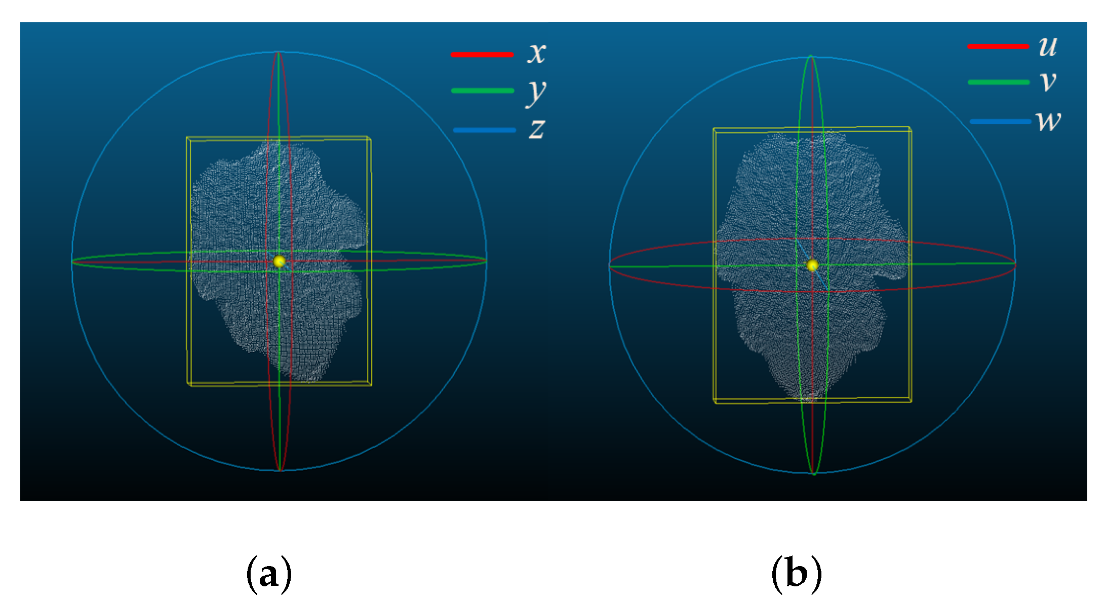
假设叶长距离大于叶宽，使用主成分分析（PCA）确定叶片的主直径轴 (𝑢,𝑣,𝑤)$(u,v,w)$ ，u 为叶长轴，v 为叶宽轴，w 为厚度轴。叶片的边界框基于 (𝑢,𝑣,𝑤)$(u,v,w)$ 坐标系构建，u 和 v 方向上与边界框相切的点为所需的关键点。

After obtaining the coordinate system, the intersection points of bounding box and leaf point cloud are extracted, which represent the maximum value of leaf extension and as the key points of measuring length and width. Figure 2a represents the coordinate system of the original point cloud, where the red straight line is the x axis, green line is the y axis, and blue line is the z axis; Figure 2b represents the coordinate system of point cloud processed by PCA, where the red straight line is the u axis, green line is the v axis, and blue line is the w axis. Assuming leaf length is greater than leaf width, u is the main axis, v is the secondary main axis, and w is the tertiary main axis. The yellow border of the 3D leaf model in Figure 2 is obtained by the bounding box method. The points intersected with the bounding box in v axis are measuring points of the leaf width, named 𝑝𝑤𝑒𝑛𝑑$p_{wend}$, 𝑝𝑤𝑠𝑡𝑎𝑟𝑡$p_{wstart}$. The point where the u axis of the bounding box intersects the bottom of the leaf is 𝑝𝑙𝑒𝑛𝑑$p_{lend}$, while the point on the other side of leaf length cannot be directly used as the point of the leaf tip. Since eggplant petiole is located in the concave surface of the point cloud, the point where the bounding box intersects with the u axis is not the petiole, so the point 𝑝𝑙𝑠𝑡𝑎𝑟𝑡$p_{lstart}$ needs to be selected manually.
在获得坐标系后，提取了边界框和叶点云的交点，这些点代表叶扩展的最大值，并作为测量长度和宽度的关键点。图 2a 表示原始点云的坐标系，其中红色直线是 x 轴，绿色线是 y 轴，蓝色线是 z 轴；图 2b 表示经过 PCA 处理后的点云坐标系，其中红色直线是 u 轴，绿色线是 v 轴，蓝色线是 w 轴。假设叶长大于叶宽，u 为主轴，v 为次主轴，w 为第三主轴。图 2 中 3D 叶模型的黄色边界是通过边界框方法获得的。与边界框在 v 轴相交的点为叶宽的测量点，命名为 𝑝𝑤𝑒𝑛𝑑$p_{wend}$ ， 𝑝𝑤𝑠𝑡𝑎𝑟𝑡$p_{wstart}$ 。边界框的 u 轴与叶底相交的点为 𝑝𝑙𝑒𝑛𝑑$p_{lend}$ ，而叶长另一侧的点不能直接用作叶尖的点。 由于茄子叶柄位于点云的凹面，因此包围盒与 u 轴相交的点不是叶柄，所以需要手动选择 𝑝𝑙𝑠𝑡𝑎𝑟𝑡$p_{lstart}$ 点。

Figure 2. Coordinate system of leaf point cloud. (a) Original coordinate system of point cloud. (b) Processed coordinate system of point cloud.
图 2. 叶点云坐标系。（a）点云原始坐标系。（b）点云处理后的坐标系。

In Figure 3a, the original point cloud is projected onto the (𝑥,𝑦,𝑧)$(x,y,z)$ coordinate system, and Figure 3b the reconstructed point cloud is projected onto the (𝑢,𝑣,𝑤)$(u,v,w)$ coordinate system. The PCA algorithm is used to process the point cloud, and the elements are mapped to the main coordinate axis, secondary main coordinate axis, and tertiary main coordinate axis. The coordinate axis of the reconstructed point cloud has regularity, which is related to the decreasing projection density of the leaf length, width, and thickness. Therefore, the reconstructed main coordinate axis u represents the length of the leaf, the secondary main coordinate axis v represents the width, and the tertiary main coordinate axis w represents the thickness.
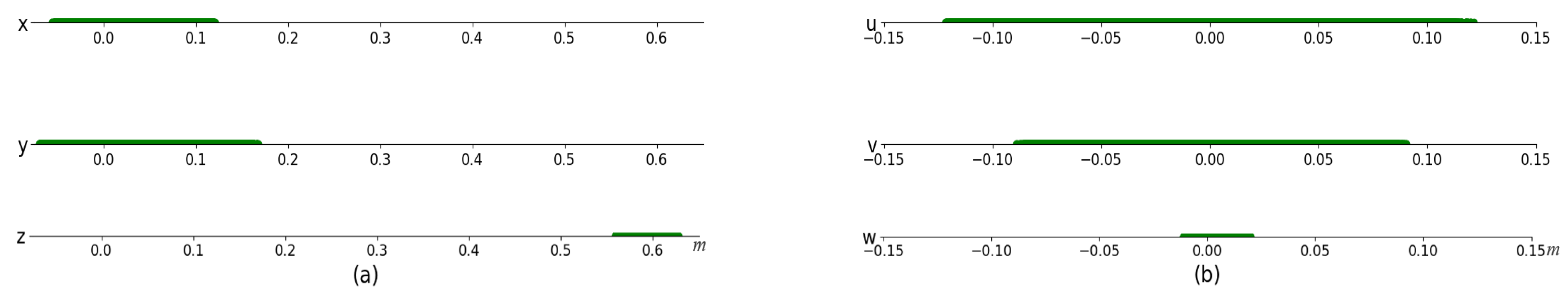
在图 3a 中，原始点云被投影到 (𝑥,𝑦,𝑧)$(x,y,z)$ 坐标系中，图 3b 中重建的点云被投影到 (𝑢,𝑣,𝑤)$(u,v,w)$ 坐标系中。使用 PCA 算法处理点云，并将元素映射到主坐标轴、次主坐标轴和三级主坐标轴。重建点云的坐标轴具有规律性，这与叶片长度、宽度和厚度的投影密度降低有关。因此，重建的主坐标轴 u 代表叶片长度，次主坐标轴 v 代表宽度，三级主坐标轴 w 代表厚度。

Figure 3. Projection of point cloud data onto the coordinate system. (a) Distribution map of the point cloud in the original coordinate system (𝑥,𝑦,𝑧)$(x,y,z)$. (b) Distribution map of the point cloud in the reconstructed coordinate system (𝑢,𝑣,𝑤)$(u,v,w)$.
图 3. 点云数据在坐标系上的投影。（a）原始坐标系下点云的分布图 (𝑥,𝑦,𝑧)$(x,y,z)$ 。（b）重建坐标系下点云的分布图 (𝑢,𝑣,𝑤)$(u,v,w)$ 。

Algorithm 1 used the PCA algorithm to reconstruct the coordinate system (𝑢,𝑣,𝑤)$(u,v,w)$ for obtaining the range of interest (RoI) of leaf and the key points of length and width.
算法 1 使用了 PCA 算法重构坐标系统 (𝑢,𝑣,𝑤)$(u,v,w)$ ，以获取叶子的感兴趣区域（RoI）以及长度和宽度的关键点。

Algorithm 1 The algorithm of obtaining the measurement points of length and width. 算法 1 获取长度和宽度测量点的算法。

Require:𝑃={𝑃1,𝑃2…𝑃𝑛},𝑃𝑖=(𝑥𝑖,𝑦𝑖,𝑧𝑖)𝑇∈𝑅,𝑖=1,2…𝑛$P=\{P_1,P_2\dots P_n\},P_i={(x_i,y_i,z_i)}^T\in R,i=1,2\dots n$     for i = 1:n do           Calculate 𝑃𝑐$\overline{P_c}$ by Equation (1)     end for     Calculate covariance matrix 𝐶𝑝$C_p$ by Equation (2)     Calculate eigenvalues and eigenvectors of 𝐶𝑝$C_p$, and express eigenvectors as the coordinate system (𝑢,𝑣,𝑤)$(u,v,w)$,     Calculate the minimum bounding box for the leaf model in the coordinate system (𝑢,𝑣,𝑤)$(u,v,w)$,     Define the reconstructed point cloud as 𝑝={𝑝1,𝑝2…𝑝𝑛}(𝑝𝑖=(𝑢𝑖,𝑣𝑖,𝑤𝑖),𝑖=(1,2…𝑛))$p=\{p_1,p_2\dots p_n\}(p_i=(u_i,v_i,w_i),i=(1,2\dots n))$,     Define the intersection point of the leaf model and the bounding box in v direction as 𝑝𝑤𝑠𝑡𝑎𝑟𝑡$p_{wstart}$, 𝑝𝑤𝑒𝑛𝑑$p_{wend}$,     Define the intersection point of the leaf model and the bounding box in u direction as 𝑝𝑙𝑒𝑛𝑑$p_{lend}$,     Define the intersection point of the leaf model in u direction as 𝑝𝑙𝑠𝑡𝑎𝑟𝑡$p_{lstart}$ manually. Ensure: 𝑝𝑙𝑠𝑡𝑎𝑟𝑡,𝑝𝑙𝑒𝑛𝑑,𝑝𝑤𝑠𝑡𝑎𝑟𝑡,𝑝𝑤𝑒𝑛𝑑∈𝑝𝑖(𝑖=1,2…𝑛)$p_{lstart},p_{lend},p_{wstart},p_{wend}\in p_i(i=1,2\dots n)$

2.2. Measurement the Length and Width of Leaf

The commonly used three-dimensional length measurement methods are the cross-section and geodesic distance methods. The cross-section method uses the key points and direction vector to find the tangent plane. In this paper, the key points have been obtained according to the bounding box technique, the length plane and width plane are perpendicular to the 𝑢𝑜𝑣$uov$ plane. The longitudinal section intersects the leaf length with a line of intersection, and the value of this line is used as the measured value of leaf length. The cross section intersects the leaf width with a line of intersection, the value of this line is used as the measured value of leaf width. The obtained length and width tangent are curves, which is consistent with the actual measurement method to obtain the curve distance from the starting point to the end point on the leaf according to the given points.
常用的三维长度测量方法有横截面和测地距离法。横截面法利用关键点和方向向量找到切平面。在本文中，根据边界框技术获得了关键点，长度平面和宽度平面垂直于 𝑢𝑜𝑣$uov$ 平面。纵向截面与叶长相交形成交线，该线的值用作叶长测量值。横截面与叶宽相交形成交线，该线的值用作叶宽测量值。获得的长宽切线是曲线，这与根据给定点从起点到终点在叶上获得曲线距离的实际测量方法一致。

The geodesic distance method is a heuristic method, in which the starting point and the end point of the measurement must be provided to find the line connecting two points according to the shortest path principle, such as A* [49], Dijkstra [50] geodetic distance method. The Dijkstra algorithm is a typical shortest path algorithm, which is used to calculate the shortest path from the starting node to the final node. The Dijkstra algorithm can obtain the optimal solution of the shortest path. For the current point on the path, A* algorithm records the cost to the source point, and the expected cost from the current point to the target point, so it is a depth-first algorithm. The commonly used heuristic functions of A* algorithm include Manhattan, Euclidean and Chebyshev distances [51]. The research object of this paper is a 3D point cloud, which can move along any direction when looking for the next target points, so the Euclidean distance is chosen as the heuristic function of A* algorithm in this paper. The space distance between points is the basis of the shortest distance. The start and end key points of the geodesic distance method are the same as those of the cross-section method, and the length and width of the leaf are calculated by the start and end key points, so there are fluctuations between adjacent point 𝑝𝑖$p_i$ and point 𝑝𝑖+1$p_{i+1}$ when searching for the shortest path.
测地距离法是一种启发式方法，其中必须提供测量的起点和终点，根据最短路径原理找到连接两点的线，例如 A* [49]、Dijkstra [50]测地距离法。Dijkstra 算法是一种典型的最短路径算法，用于计算从起始节点到最终节点的最短路径。Dijkstra 算法可以获得最短路径的最优解。对于路径上的当前点，A*算法记录到源点的成本和从当前点到目标点的预期成本，因此它是一种深度优先算法。A*算法常用的启发式函数包括曼哈顿距离、欧几里得距离和切比雪夫距离[51]。本文的研究对象是 3D 点云，在寻找下一个目标点时可以沿任何方向移动，因此本文选择欧几里得距离作为 A*算法的启发式函数。点之间的空间距离是最短距离的基础。 起始和终止关键点与横截面方法相同，叶子的长度和宽度通过起始和终止关键点计算，因此在寻找最短路径时，相邻点 𝑝𝑖$p_i$ 和点 𝑝𝑖+1$p_{i+1}$ 之间存在波动。

In this paper, based on the cross-section method, the direction of the section is not perpendicular to the coordinate system, but the plane is constructed according to the point on the leaf closest to the center of the starting point and the end point. This paper proposes to use the cutting-plane method to obtain the intersection line of the leaf as the basis for measuring the length and width. For the leaf length, the starting point 𝑝𝑙𝑠𝑡𝑎𝑟𝑡$p_{lstart}$ and end point 𝑝𝑙𝑒𝑛𝑑$p_{lend}$ were obtained, but to determine a plane, three points which are not on the same straight line are required, so the third point is needed to construct the three-dimensional plane. Similarly, for the leaf width, the starting point 𝑝𝑤𝑠𝑡𝑎𝑟𝑡$p_{wstart}$ and the end point 𝑝𝑤𝑒𝑛𝑑$p_{wend}$ have been obtained by bounding box technology, and the third point is also needed to construct the width plane. The method proposed in this paper is not to calculate the length and width of the leaf according to the point cloud perpendicular to the coordinate system 𝑢𝑜𝑣$uov$, and the process of coordinate system transformation can be omitted. It needs to specify the starting point and end point to calculate the target points for the leaf point cloud, then determine the tangent plane of length and width.
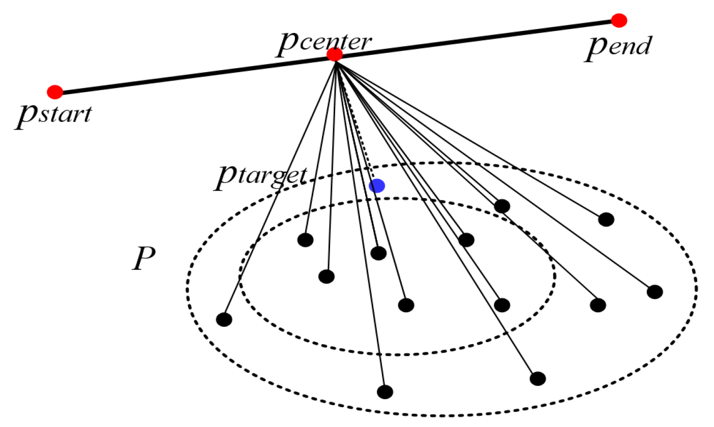
在这篇论文中，基于横截面法，截面方向并非垂直于坐标系，而是根据叶子上离起点和终点最近的点构建平面。本文提出使用切割平面法获取叶子交线作为测量长度和宽度的基础。对于叶子长度，获得了起点 𝑝𝑙𝑠𝑡𝑎𝑟𝑡$p_{lstart}$ 和终点 𝑝𝑙𝑒𝑛𝑑$p_{lend}$ ，但确定一个平面需要三个不在同一直线上的点，因此需要第三个点来构建三维平面。同样，对于叶子宽度，通过边界框技术获得了起点 𝑝𝑤𝑠𝑡𝑎𝑟𝑡$p_{wstart}$ 和终点 𝑝𝑤𝑒𝑛𝑑$p_{wend}$ ，也需要第三个点来构建宽度平面。本文提出的方法不是根据垂直于坐标系的点云 𝑢𝑜𝑣$uov$ 来计算叶子的长度和宽度，可以省略坐标系转换的过程。 需要指定起点和终点来计算叶点云的目标点，然后确定长度和宽度的切平面。

In order to obtain the third point, the midpoint of the line between the starting point 𝑝𝑙𝑠𝑡𝑎𝑟𝑡$p_{lstart}$ and the end point 𝑝𝑙𝑒𝑛𝑑$p_{lend}$ is set as 𝑝𝑙𝑐𝑒𝑛𝑡𝑒𝑟$p_{lcenter}$ in Equation (3). The point closest to 𝑝𝑙𝑐𝑒𝑛𝑡𝑒𝑟$p_{lcenter}$ on the leaf point cloud is selected as the third point 𝑝𝑙𝑡𝑎𝑟𝑔𝑒𝑡$p_{ltarget}$ on the cutting plane in Equation (4). The target point 𝑝𝑙𝑡𝑎𝑟𝑔𝑒𝑡$p_{ltarget}$ selected in this way can ensure the closest distance to the point 𝑝𝑙𝑐𝑒𝑛𝑡𝑒𝑟$p_{lcenter}$, and the three points 𝑝𝑙𝑠𝑡𝑎𝑟𝑡$p_{lstart}$, 𝑝𝑙𝑒𝑛𝑑$p_{lend}$ and 𝑝𝑙𝑡𝑎𝑟𝑔𝑒𝑡$p_{ltarget}$ constituted the plane from the three-dimensional leaf model.
为了获得第三点，将起点 𝑝𝑙𝑠𝑡𝑎𝑟𝑡$p_{lstart}$ 和终点 𝑝𝑙𝑒𝑛𝑑$p_{lend}$ 之间的线段中点设为方程（3）中的 𝑝𝑙𝑐𝑒𝑛𝑡𝑒𝑟$p_{lcenter}$ 。在叶点云上选择距离 𝑝𝑙𝑐𝑒𝑛𝑡𝑒𝑟$p_{lcenter}$ 最近的点作为方程（4）中切割平面上的第三点 𝑝𝑙𝑡𝑎𝑟𝑔𝑒𝑡$p_{ltarget}$ 。以这种方式选择的靶点 𝑝𝑙𝑡𝑎𝑟𝑔𝑒𝑡$p_{ltarget}$ 可以确保与点 𝑝𝑙𝑐𝑒𝑛𝑡𝑒𝑟$p_{lcenter}$ 的距离最近，而三个点 𝑝𝑙𝑠𝑡𝑎𝑟𝑡$p_{lstart}$ 、 𝑝𝑙𝑒𝑛𝑑$p_{lend}$ 和 𝑝𝑙𝑡𝑎𝑟𝑔𝑒𝑡$p_{ltarget}$ 构成了三维叶模型构成的平面。

𝑝𝑙𝑐𝑒𝑛𝑡𝑒𝑟=(𝑝𝑙𝑠𝑡𝑎𝑟𝑡+𝑝𝑙𝑒𝑛𝑑)2$$\begin{array}{cc}\hfill p_{lcenter}& =\frac{(p_{lstart}+p_{lend})}{2}\hfill \end{array}$$

(3)

𝑝𝑙𝑡𝑎𝑟𝑔𝑒𝑡=𝑃𝑚𝑖𝑛{𝑑(𝑝𝑙𝑐𝑒𝑛𝑡𝑒𝑟,𝑝𝑖)}$$\begin{array}{cc}\hfill p_{ltarget}& =P_{min}\left\{d(p_{lcenter},p_i)\right\}\hfill \end{array}$$

(4)

where, 𝑃𝑚𝑖𝑛$P_{min}$ denotes the coordinates of the point with the smallest distance between 𝑝𝑙𝑐𝑒𝑛𝑡𝑒𝑟$p_{lcenter}$ and 𝑝𝑖$p_i$, and d denotes the Euclidean distance of two points. Similarly, when calculating the width tangent plane, the midpoint of the line between the starting point 𝑝𝑤𝑠𝑡𝑎𝑟𝑡$p_{wstart}$ and the end point 𝑝𝑤𝑒𝑛𝑑$p_{wend}$ is 𝑝𝑤𝑐𝑒𝑛𝑡𝑒𝑟$p_{wcenter}$ in Equation (5). The point closest to 𝑝𝑤𝑐𝑒𝑛𝑡𝑒𝑟$p_{wcenter}$ is selected as 𝑝𝑤𝑡𝑎𝑟𝑔𝑒𝑡$p_{wtarget}$ on the leaf model in Equation (6).
在式中， 𝑃𝑚𝑖𝑛$P_{min}$ 表示 𝑝𝑙𝑐𝑒𝑛𝑡𝑒𝑟$p_{lcenter}$ 和 𝑝𝑖$p_i$ 之间距离最小的点的坐标，d 表示两点之间的欧几里得距离。类似地，在计算宽度切平面时，方程（5）中的起点 𝑝𝑤𝑠𝑡𝑎𝑟𝑡$p_{wstart}$ 和终点 𝑝𝑤𝑒𝑛𝑑$p_{wend}$ 之间的线段中点为 𝑝𝑤𝑐𝑒𝑛𝑡𝑒𝑟$p_{wcenter}$ 。在方程（6）的叶模型中，选择距离 𝑝𝑤𝑐𝑒𝑛𝑡𝑒𝑟$p_{wcenter}$ 最近的点作为 𝑝𝑤𝑡𝑎𝑟𝑔𝑒𝑡$p_{wtarget}$ 。

𝑝𝑤𝑐𝑒𝑛𝑡𝑒𝑟=(𝑝𝑤𝑠𝑡𝑎𝑟𝑡+𝑝𝑤𝑒𝑛𝑑)2$$\begin{array}{cc}\hfill p_{wcenter}& =\frac{(p_{wstart}+p_{wend})}{2}\hfill \end{array}$$

(5)

𝑝𝑤𝑡𝑎𝑟𝑔𝑒𝑡=𝑃𝑚𝑖𝑛{𝑑(𝑝𝑤𝑐𝑒𝑛𝑡𝑒𝑟,𝑝𝑖)}$$\begin{array}{cc}\hfill p_{wtarget}& =P_{min}\left\{d(p_{wcenter},p_i)\right\}\hfill \end{array}$$

(6)

In Figure 4, the red points, respectively, represent 𝑝𝑠𝑡𝑎𝑟𝑡$p_{start}$, 𝑝𝑒𝑛𝑑$p_{end}$, and 𝑝𝑐𝑒𝑛𝑡𝑒𝑟$p_{center}$, while black points represent the 3D leaf model. The point with the smallest distance to 𝑝𝑐𝑒𝑛𝑡𝑒𝑟$p_{center}$ is selected as 𝑝𝑡𝑎𝑟𝑔𝑒𝑡$p_{target}$, which is represented in blue.
在图 4 中，红色点分别代表 𝑝𝑠𝑡𝑎𝑟𝑡$p_{start}$ 、 𝑝𝑒𝑛𝑑$p_{end}$ 和 𝑝𝑐𝑒𝑛𝑡𝑒𝑟$p_{center}$ ，而黑色点代表 3D 叶片模型。距离 𝑝𝑐𝑒𝑛𝑡𝑒𝑟$p_{center}$ 最近的点被选为 𝑝𝑡𝑎𝑟𝑔𝑒𝑡$p_{target}$ ，用蓝色表示。

Figure 4. Determination of the target point by starting and end point.
图 4. 由起点和终点确定目标点。

For the section of leaf length, the three points of 𝑝𝑙𝑠𝑡𝑎𝑟𝑡$p_{lstart}$, 𝑝𝑙𝑒𝑛𝑑$p_{lend}$ and 𝑝𝑙𝑐𝑒𝑛𝑡𝑒𝑟$p_{lcenter}$ are on the same straight line, then 𝑝𝑙𝑡𝑎𝑟𝑔𝑒𝑡$p_{ltarget}$ and 𝑝𝑙𝑠𝑡𝑎𝑟𝑡$p_{lstart}$ and 𝑝𝑒𝑛𝑑$p_{end}$ are not on the same straight line, so according to the plane equation, it can be guaranteed that the three points determine a plane. For the section of width, 𝑝𝑤𝑡𝑎𝑟𝑔𝑒𝑡$p_{wtarget}$ and 𝑝𝑤𝑠𝑡𝑎𝑟𝑡$p_{wstart}$ and 𝑝𝑤𝑒𝑛𝑑$p_{wend}$ are not in a straight line, so here it can be guaranteed that three points define a plane. This process is to compare the distance between the point set 𝑝𝑖$p_i$ and 𝑝𝑐𝑒𝑛𝑡𝑒𝑟$p_{center}$, and select the point p corresponding to the smallest distance as the point 𝑝𝑡𝑎𝑟𝑔𝑒𝑡$p_{target}$. The purpose is to determine a plane through a line and point, and cut a curve through the plane and leaf point cloud surface.
对于叶片长度的部分，点 𝑝𝑙𝑠𝑡𝑎𝑟𝑡$p_{lstart}$ 、 𝑝𝑙𝑒𝑛𝑑$p_{lend}$ 和 𝑝𝑙𝑐𝑒𝑛𝑡𝑒𝑟$p_{lcenter}$ 在同一直线上，而点 𝑝𝑙𝑡𝑎𝑟𝑔𝑒𝑡$p_{ltarget}$ 、 𝑝𝑙𝑠𝑡𝑎𝑟𝑡$p_{lstart}$ 和 𝑝𝑒𝑛𝑑$p_{end}$ 不在同一直线上，因此根据平面方程，可以保证这三个点确定一个平面。对于宽度部分，点 𝑝𝑤𝑡𝑎𝑟𝑔𝑒𝑡$p_{wtarget}$ 、 𝑝𝑤𝑠𝑡𝑎𝑟𝑡$p_{wstart}$ 和 𝑝𝑤𝑒𝑛𝑑$p_{wend}$ 不在同一直线上，因此可以保证三个点定义一个平面。这个过程是为了比较点集 𝑝𝑖$p_i$ 和 𝑝𝑐𝑒𝑛𝑡𝑒𝑟$p_{center}$ 之间的距离，并选择对应最小距离的点 p 作为点 𝑝𝑡𝑎𝑟𝑔𝑒𝑡$p_{target}$ 。目的是通过一条直线和一个点确定一个平面，并通过平面和叶片点云表面切割一条曲线。

The length and width section of the leaf obtained by the traditional cross-section method is shown in Figure 5a, the coordinate system was reconstructed according to the PCA method, and the length and width planes are perpendicular to the coordinate plane 𝑢𝑜𝑣$uov$. For the width section, suppose the equation is 𝐴𝑤𝑥+𝐵𝑤𝑦+𝐶𝑤𝑧+𝐷𝑤=0$A_{w}x+B_{w}y+C_{w}z+D_w=0$. The plane 𝐹𝑤$F_w$ through three points that are not on the same line in the equation are 𝑝𝑤𝑠𝑡𝑎𝑟𝑡$p_{wstart}$, 𝑝𝑤𝑡𝑎𝑟𝑔𝑒𝑡$p_{wtarget}$, and 𝑝𝑤𝑒𝑛𝑑$p_{wend}$. The transverse plane tangent of the leaf is shown in Figure 5b. Suppose the length plane equation is 𝐴𝑙𝑥+𝐵𝑙𝑦+𝐶𝑙𝑧+𝐷𝑙=0$A_{l}x+B_{l}y+C_{l}z+D_l=0$. The plane 𝐹𝑙$F_l$ through three points that are not on the same line in the equation are 𝑝𝑙𝑠𝑡𝑎𝑟𝑡$p_{lstart}$, 𝑝𝑙𝑡𝑎𝑟𝑔𝑒𝑡$p_{ltarget}$, and 𝑝𝑙𝑒𝑛𝑑$p_{lend}$. The plane tangent of the leaf length in Figure 5c. The section intersects the leaf length with a line, as 𝑙𝑙$l_l$. Similarly, the section intersects the leaf width with a line, as 𝑙𝑤$l_w$.
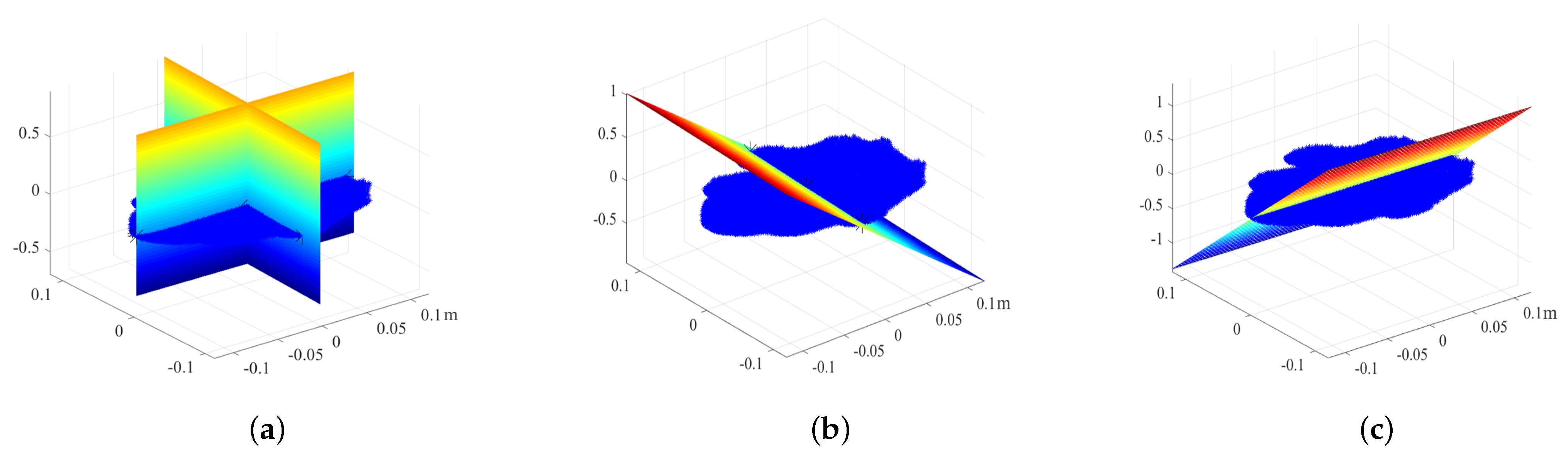
图 5a 显示了通过传统横切法获得的叶片长度和宽度部分，坐标系统根据主成分分析（PCA）方法重建，长度和宽度平面垂直于坐标平面 𝑢𝑜𝑣$uov$ 。对于宽度部分，假设方程为 𝐴𝑤𝑥+𝐵𝑤𝑦+𝐶𝑤𝑧+𝐷𝑤=0$A_{w}x+B_{w}y+C_{w}z+D_w=0$ 。通过方程中不在同一直线上的三个点 𝑝𝑤𝑠𝑡𝑎𝑟𝑡$p_{wstart}$ 、 𝑝𝑤𝑡𝑎𝑟𝑔𝑒𝑡$p_{wtarget}$ 和 𝑝𝑤𝑒𝑛𝑑$p_{wend}$ 确定的平面 𝐹𝑤$F_w$ 。叶片的横切面在图 5b 中显示。假设长度平面方程为 𝐴𝑙𝑥+𝐵𝑙𝑦+𝐶𝑙𝑧+𝐷𝑙=0$A_{l}x+B_{l}y+C_{l}z+D_l=0$ 。通过方程中不在同一直线上的三个点 𝑝𝑙𝑠𝑡𝑎𝑟𝑡$p_{lstart}$ 、 𝑝𝑙𝑡𝑎𝑟𝑔𝑒𝑡$p_{ltarget}$ 和 𝑝𝑙𝑒𝑛𝑑$p_{lend}$ 确定的平面 𝐹𝑙$F_l$ 是叶片长度的切平面。图 5c 中显示了与叶片长度相交的截面线，如 𝑙𝑙$l_l$ 。类似地，截面线与叶片宽度相交，如 𝑙𝑤$l_w$ 。

Figure 5. Obtaining spatial length and width planes of leaf. (a) Spatial planes of length and width by cross-section method. (b) Spatial plane of width according to this paper. (c) Spatial plane of length according to this paper.
图 5. 获取叶片的空间长度和宽度平面。（a）通过横切法获得的长度和宽度空间平面。（b）根据本文获得的宽度空间平面。（c）根据本文获得的长度空间平面。

The length and width cut planes obtained by this paper are not perpendicular to the coordinate plane. The essence of our method is to use the tangent plane to cut the model and obtain the point on the intersection line as the basis for calculating the length and width. The leaf model intersects with the length and width planes, which are used to measure the distance of length and width in Algorithm 2.
该文获得的长度和宽度切割平面与坐标平面不垂直。我们方法的核心是利用切平面切割模型，并将交线上的点作为计算长度和宽度的基础。叶模型与长度和宽度平面相交，这些平面用于在算法 2 中测量长度和宽度。

Algorithm 2 The algorithm of calculating leaf length and width. 算法 2 计算叶长和叶宽的算法。

Process of calculating leaf length 计算叶片长度的过程 Require: 𝑃={𝑝1,𝑝2…𝑝𝑛},𝑖=(1,2…𝑛)$P=\{p_1,p_2\dots p_n\},i=(1,2\dots n)$  需要： 𝑃={𝑝1,𝑝2…𝑝𝑛},𝑖=(1,2…𝑛)$P=\{p_1,p_2\dots p_n\},i=(1,2\dots n)$     Calculate the midpoint 𝑝𝑙𝑐𝑒𝑛𝑡𝑒𝑟$p_{lcenter}$ of line 𝑙𝑙$l_l$ using Equation (3). 计算直线 𝑙𝑙$l_l$ 的中点 𝑝𝑙𝑐𝑒𝑛𝑡𝑒𝑟$p_{lcenter}$ ，使用公式（3）。     for i = 1:n do 对于 i = 1 到 n 循环           Calculate the distance between 𝑝𝑖$p_i$ and 𝑝𝑙𝑐$p_{lc}$ as 𝑑𝑙𝑖$d_{li}$, 计算 𝑝𝑖$p_i$ 与 𝑝𝑙𝑐$p_{lc}$ 之间的距离为 𝑑𝑙𝑖$d_{li}$ ，           Find 𝑑𝑙𝑚𝑖𝑛=min𝑑𝑙𝑖$d_{lmin}=min{d}_{li}$, and the keypoint 𝑝𝑙𝑡𝑎𝑟𝑔𝑒𝑡$p_{ltarget}$ using Equation (4). 找到 𝑑𝑙𝑚𝑖𝑛=min𝑑𝑙𝑖$d_{lmin}=min{d}_{li}$ ，并使用公式（4）确定关键点 𝑝𝑙𝑡𝑎𝑟𝑔𝑒𝑡$p_{ltarget}$ 。     end for     Calculate the cutting plane of 𝑝𝑙𝑠𝑡𝑎𝑟𝑡,𝑝𝑙𝑒𝑛𝑑,𝑝𝑙𝑡𝑎𝑟𝑔𝑒𝑡$p_{lstart},p_{lend},p_{ltarget}$ as 𝐴𝑙𝑥+𝐵𝑙𝑦+𝐶𝑙𝑧+𝐷𝑙=0$A_{lx}+B_{ly}+C_{lz}+D_l=0$, 计算 𝑝𝑙𝑠𝑡𝑎𝑟𝑡,𝑝𝑙𝑒𝑛𝑑,𝑝𝑙𝑡𝑎𝑟𝑔𝑒𝑡$p_{lstart},p_{lend},p_{ltarget}$ 的切割平面为 𝐴𝑙𝑥+𝐵𝑙𝑦+𝐶𝑙𝑧+𝐷𝑙=0$A_{lx}+B_{ly}+C_{lz}+D_l=0$ ，     Define the tangent point set of leaf model and cutting plane as the length. 定义叶模型切点集和切割平面的长度。 Ensure:  请提供需要翻译的源文本，以便我进行翻译     𝑝𝑙𝑘∈$p_{lk}\in$ tangent point set 𝑘=1,2…𝑗$k=1,2\dots j$ 𝑝𝑙𝑘∈$p_{lk}\in$ 切点集 𝑘=1,2…𝑗$k=1,2\dots j$       Process of calculating leaf width 计算叶片宽度过程 Require: 𝑃={𝑝1,𝑝2…𝑝𝑛},𝑖=(1,2…𝑛)$P=\{p_1,p_2\dots p_n\},i=(1,2\dots n)$  需要： 𝑃={𝑝1,𝑝2…𝑝𝑛},𝑖=(1,2…𝑛)$P=\{p_1,p_2\dots p_n\},i=(1,2\dots n)$     Calculate the midpoint 𝑝𝑤𝑐𝑒𝑛𝑡𝑒𝑟$p_{wcenter}$ of line 𝑙𝑤$l_w$ using Equation (5). 计算直线 𝑙𝑤$l_w$ 的中点 𝑝𝑤𝑐𝑒𝑛𝑡𝑒𝑟$p_{wcenter}$ ，使用公式（5）。     for i = 1:n do 对于 i = 1 到 n 循环           Calculate the distance between 𝑝𝑖$p_i$ and 𝑝𝑤𝑐$p_{wc}$ as 𝑑𝑤𝑖$d_{wi}$, 计算 𝑝𝑖$p_i$ 与 𝑝𝑤𝑐$p_{wc}$ 之间的距离为 𝑑𝑤𝑖$d_{wi}$ ，           Find 𝑑𝑤𝑚𝑖𝑛=min𝑑𝑤𝑖$d_{wmin}=min{d}_{wi}$, and the keypoint 𝑝𝑤𝑡𝑎𝑟𝑔𝑒𝑡$p_{wtarget}$ using Equation (6). 找到 𝑑𝑤𝑚𝑖𝑛=min𝑑𝑤𝑖$d_{wmin}=min{d}_{wi}$ ，并使用公式（6）确定关键点 𝑝𝑤𝑡𝑎𝑟𝑔𝑒𝑡$p_{wtarget}$ 。     end for     Calculate the cutting plane of 𝑝𝑤𝑠𝑡𝑎𝑟𝑡,𝑝𝑤𝑒𝑛𝑑,𝑝𝑤𝑡𝑎𝑟𝑔𝑒𝑡$p_{wstart},p_{wend},p_{wtarget}$ as 𝐴𝑤𝑥+𝐵𝑤𝑦+𝐶𝑤𝑧+𝐷𝑤=0$A_{wx}+B_{wy}+C_{wz}+D_w=0$, 计算 𝑝𝑤𝑠𝑡𝑎𝑟𝑡,𝑝𝑤𝑒𝑛𝑑,𝑝𝑤𝑡𝑎𝑟𝑔𝑒𝑡$p_{wstart},p_{wend},p_{wtarget}$ 的切割平面为 𝐴𝑤𝑥+𝐵𝑤𝑦+𝐶𝑤𝑧+𝐷𝑤=0$A_{wx}+B_{wy}+C_{wz}+D_w=0$ ，     Define the tangent point set of leaf model and cutting plane as the width. 定义叶模型的切点集和切割平面为宽度。 Ensure:  请提供需要翻译的源文本，以便我进行翻译     𝑝𝑤𝑘∈$p_{wk}\in$ tangent point set 𝑘=1,2…𝑙$k=1,2\dots l$ 𝑝𝑤𝑘∈$p_{wk}\in$ 切点集 𝑘=1,2…𝑙$k=1,2\dots l$

Figure 6 shows the length and width points of eggplant leaves obtained by geodesic distance and cross-section methods. A* and Dijkstra methods were used for geodesic distance method. The starting point and ending point of geodesic distance method and cross-section method are the same, that is 𝑃𝑙𝑠𝑡𝑎𝑟𝑡$P_{lstart}$, 𝑝𝑤𝑠𝑡𝑎𝑟𝑡$p_{wstart}$, 𝑝𝑙𝑒𝑛𝑑$p_{lend}$, 𝑝𝑤𝑒𝑛𝑑$p_{wend}$. The red line represents the width in Figure 6a and length Figure 6e of the leaf obtained by A* method, the blue line represents the width in Figure 6b and length Figure 6f of the leaf obtained by the Dijkstra method, and the orange line represents the width in Figure 6c and length Figure 6g of the leaf obtained by the cross-section method. The green line represents the width in Figure 6d and length Figure 6h of the leaf obtained by our method. When the starting point and end point are given, our method obtains the key points through the starting and end point.

Figure 6. Obtaining the point sets of leaf length and width. (a) Obtaining the key point set of width by A* algorithm. (b) Obtaining the key point set of width by Dijkstra algorithm. (c) Obtaining the key point set of width by cross-section algorithm. (d) Obtaining the key point set of width by our method. (e) Obtaining the key point set of length by A* algorithm. (f) Obtaining the key point set of length by Dijkstra algorithm. (g) Obtaining the key point set of length by cross-section algorithm. (h) Obtaining the key point set of length by our method.
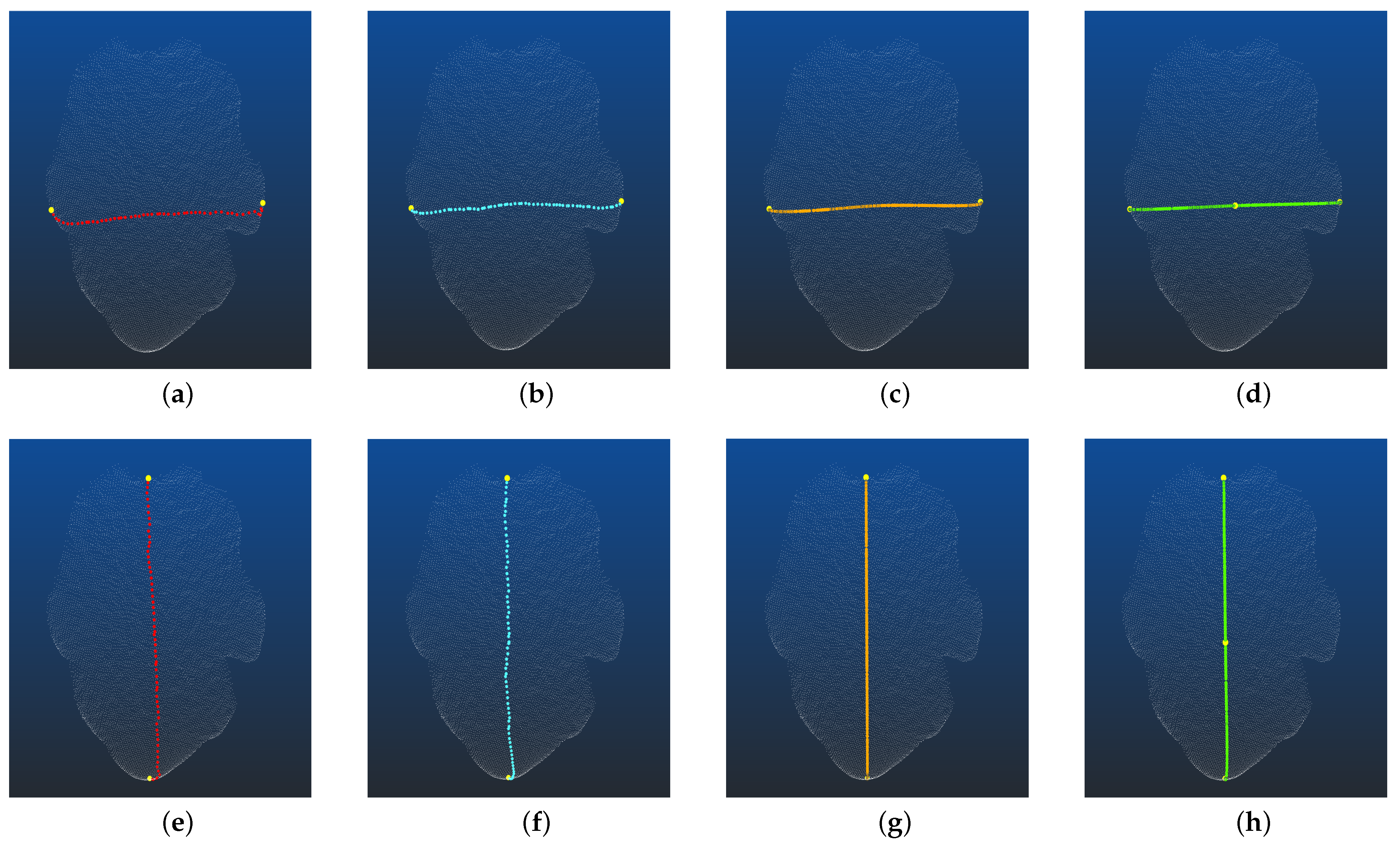
图 6. 获取叶长和叶宽的点集。（a）通过 A*算法获取宽度关键点集。（b）通过 Dijkstra 算法获取宽度关键点集。（c）通过截面算法获取宽度关键点集。（d）通过我们的方法获取宽度关键点集。（e）通过 A*算法获取长度关键点集。（f）通过 Dijkstra 算法获取长度关键点集。（g）通过截面算法获取长度关键点集。（h）通过我们的方法获取长度关键点集。

The geodetic distance method, cross-section method, and the method of this paper have the same starting and end points. The points obtained by A*, Dijkstra method are all on the original point cloud, and the shortest distance from the starting point to the end point obtaining according to the distance between each point of the leaf model. Therefore, the geodetic distance method requires more time, and the time complexity of the Dijkstra method is 𝒪(𝑛2)${\mathcal{O}}_{\left(n^2\right)}$ [52]. The essence of the cross-section method and this paper is to take the intersection point of the section and the model as the key points. The principle of the cross-section method to obtain the plane is based on the starting point, the end point and the vector perpendicular to the coordinate plane. The principle of this paper is based on the starting point, end point and target points. Therefore, in Figure 6d,h, there is starting point, end point and target point indicated by yellow dots.
大地测量距离法、横截面法和本文的方法具有相同的起点和终点。A*算法和 Dijkstra 算法得到的所有点都在原始点云上，根据叶模型中每一点之间的距离获得从起点到终点的最短距离。因此，大地测量距离法需要更多时间，Dijkstra 算法的时间复杂度为 𝒪(𝑛2)${\mathcal{O}}_{\left(n^2\right)}$ [ 52]。横截面法和本文的本质是将横截面与模型的交点作为关键点。横截面法获得平面的原理基于起点、终点和垂直于坐标平面的向量。本文的原理基于起点、终点和目标点。因此，在图 6d、h 中，有黄色圆点标记的起点、终点和目标点。

3. Results

In this paper, 20 three-dimensional eggplant leaves were taken as experimental objects, and obtain the key points of each model 𝑝𝑙𝑠𝑡𝑎𝑟𝑡$p_{lstart}$, 𝑝𝑙𝑒𝑛𝑑$p_{lend}$, 𝑝𝑤𝑠𝑡𝑎𝑟𝑡$p_{wstart}$ and 𝑝𝑤𝑒𝑛𝑑$p_{wend}$. After obtaining the key points 𝑝𝑙𝑡𝑎𝑟𝑔𝑒𝑡$p_{ltarget}$ and 𝑝𝑤𝑡𝑎𝑟𝑔𝑒𝑡$p_{wtarget}$, the length and width were calculated by A*, Dijkstra, cross-section and methods proposed in this paper. For the key point set of cutting plane 𝑝𝑘$p_k$, it needs to be connected and measured between two adjacent points 𝑝𝑘𝑖$p_{ki}$ and 𝑝𝑘(𝑖+1)$p_{k(i+1)}$ by spatial distance. Figure 7 shows the measurement values of length(or width) comparison between our method with A* algorithm, Dijkstra algorithm and cross-section method under certain practical measurement values. The points of the coordinate axis represent the estimated values obtained by the algorithms, while the horizontal coordinate axis represents the actual width and length values. From Figure 7a–d, the method proposed in this paper was compared with A*, Dijkstra and cross-section methods, and the differences with actual values.
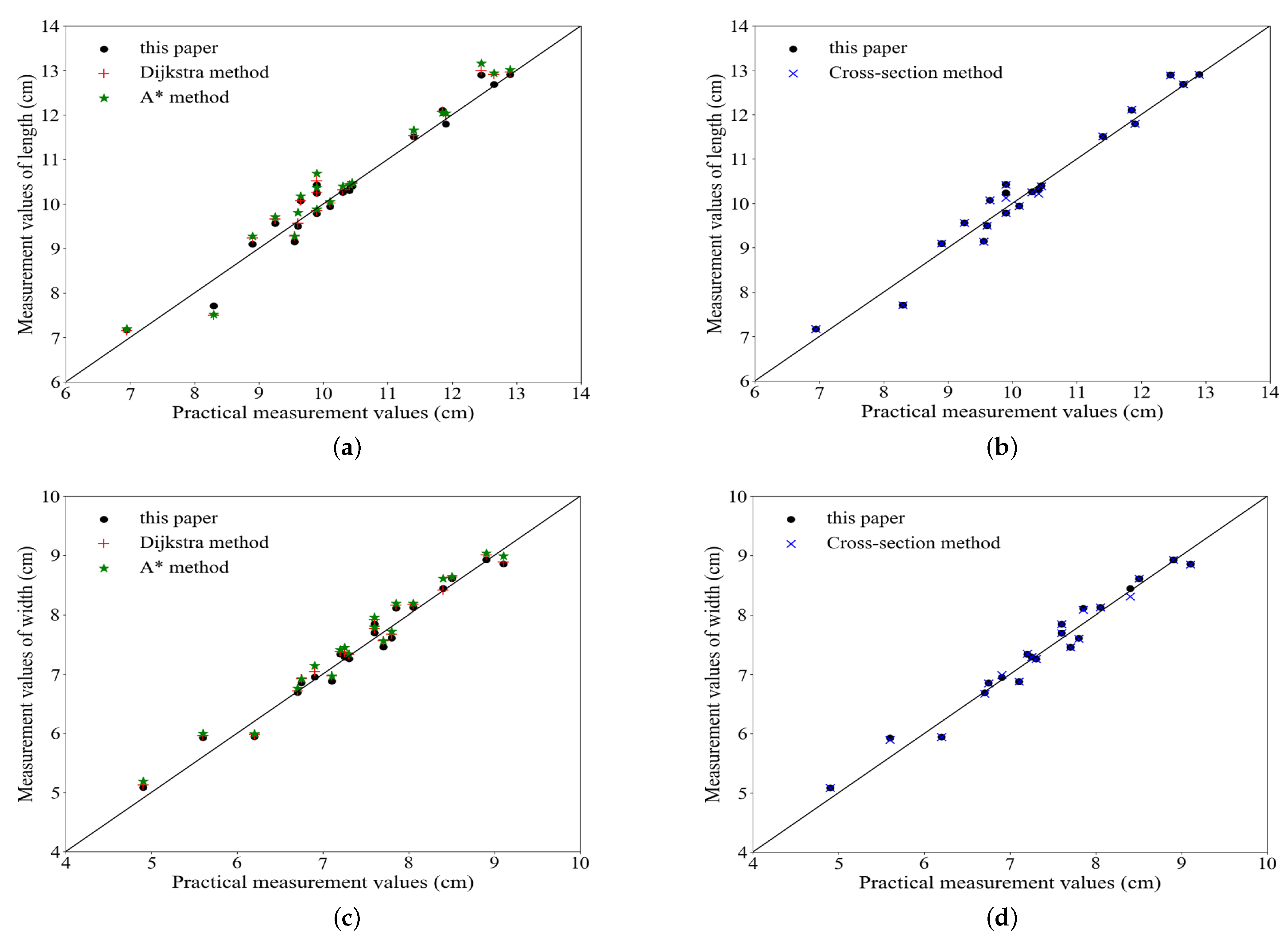
在这篇论文中，选取了 20 个三维茄子叶片作为实验对象，并获得了每个模型的要点 𝑝𝑙𝑠𝑡𝑎𝑟𝑡$p_{lstart}$ 、 𝑝𝑙𝑒𝑛𝑑$p_{lend}$ 、 𝑝𝑤𝑠𝑡𝑎𝑟𝑡$p_{wstart}$ 和 𝑝𝑤𝑒𝑛𝑑$p_{wend}$ 。在获得要点 𝑝𝑙𝑡𝑎𝑟𝑔𝑒𝑡$p_{ltarget}$ 和 𝑝𝑤𝑡𝑎𝑟𝑔𝑒𝑡$p_{wtarget}$ 后，通过 A*、Dijkstra、横截面以及本文提出的方法计算长度和宽度。对于切割平面 𝑝𝑘$p_k$ 的要点集，需要通过空间距离连接并测量两个相邻点 𝑝𝑘𝑖$p_{ki}$ 和 𝑝𝑘(𝑖+1)$p_{k(i+1)}$ 。图 7 显示了在特定实际测量值下，与 A*算法、Dijkstra 算法和横截面方法相比，我们方法测量长度（或宽度）的值。坐标轴的点代表算法获得的估计值，而水平坐标轴代表实际的宽度和长度值。从图 7a-d 可以看出，本文提出的方法与 A*、Dijkstra 和横截面方法进行了比较，并显示了与实际值的差异。

Figure 7. Comparison of the length and width values measured by algorithms with actual values. (a) Comparison of the geodesic distance method with this paper on leaf length. (b) Comparison of cross-section method with this paper on leaf length. (c) Comparison of geodesic distance method with this paper on leaf width. (d) Comparison of cross-section method with this paper on leaf width.
图 7. 算法测量的长度和宽度值与实际值的比较。（a）与本文关于叶片长度的测地距离方法的比较。（b）与本文关于叶片长度的横截面积方法的比较。（c）与本文关于叶片宽度的测地距离方法的比较。（d）与本文关于叶片宽度的横截面积方法的比较。

The coefficients of determination (𝑅2$R^2$) of 20 groups of data were calculated to compare the accuracy of each method, where the length calculated by bthe A* method compared with the actual length was 0.930; the value of length calculated by the Dijkstra method compared with the actual length was 0.949; the value of length calculated by the cross-section method compared with the actual length was 0.963; the value of length calculated by this paper compared with the actual length was 0.962; the value of width calculated by the A* method compared with the actual width was 0.956; the value of width calculated by the Dijkstra method and compared with actual width was 0.966; the value of width calculated by the cross-section method compared with the actual width was 0.970; the value of width calculated by this paper compared with the actual width was 0.970; Compared with the errors of the geodetic distance method and cross-section method, this paper’s method with actual values tested in this paper were all within the acceptable range of the study, so these methods can be used to measure the length and width of the leaf. But in terms of time complexity, the geodesic distance needs extra time to compare the distance between points, so the cross-section method and the algorithm in this paper have low time complexity. The algorithm in this paper needs one traversal to find the target point, and the time complexity is 𝒪(𝑛)${\mathcal{O}}_{\left(n\right)}$. In terms of algorithm complexity, the cross-section method needs to reconstruct the coordinate system to obtain the vector. The algorithm in this paper constructs a spatial plane based on three points that are not on the same straight line, which does not require the process of reconstructing the coordinate system. The accuracy of this paper and cross-section method are higher than geodetic distance method, because all points of the geodetic distance method must be in the model when selecting the shortest path. Our method is similar to the cross-section method, which are both cutting the model by plane, and the key points are obtained through the tangent line.
确定系数（ 𝑅2$R^2$ ）计算了 20 组数据，以比较每种方法的准确性，其中 A*方法计算出的长度与实际长度相比为 0.930；Dijkstra 方法计算出的长度与实际长度相比为 0.949；横截面方法计算出的长度与实际长度相比为 0.963；本文方法计算出的长度与实际长度相比为 0.962；A*方法计算出的宽度与实际宽度相比为 0.956；Dijkstra 方法计算出的宽度与实际宽度相比为 0.966；横截面方法计算出的宽度与实际宽度相比为 0.970；本文方法计算出的宽度与实际宽度相比为 0.970；与大地距离法和横截面法的误差相比，本文中测试的实际值均在研究的可接受范围内，因此这些方法可以用来测量叶片的长度和宽度。 但就时间复杂度而言，测地距离需要额外的时间来比较点之间的距离，因此横截法以及本文中的算法具有较低的时间复杂度。本文中的算法需要一次遍历来找到目标点，其时间复杂度为 𝒪(𝑛)${\mathcal{O}}_{\left(n\right)}$ 。在算法复杂度方面，横截法需要重建坐标系以获得向量。本文中的算法基于不在同一直线上的三个点构建空间平面，无需重建坐标系的流程。本文的方法和横截法的精度高于测地距离法，因为选择最短路径时，测地距离法的所有点都必须在模型中。我们的方法与横截法类似，都是通过平面切割模型，关键点通过切线获得。

Compared with a two-dimensional image, a three-dimensional point cloud contains spatial information of the object. This article proves that the geodetic distance and cross-section methods are also suitable for the measurement of the three-dimensional leaf model.
与二维图像相比，三维点云包含物体的空间信息。本文证明，大地测量距离法和横截面法也适用于三维叶片模型的测量。

4. Discussion and Conclusions

The geodetic distance method is the process of finding the key points at the shortest distance from the starting point to end point on the original point cloud. It uses the distance relationship between points on the point cloud as the basis for obtaining the shortest distance in the next step. The time complexity of the Dijkstra method is 𝒪(𝑛2)${\mathcal{O}}_{\left(n^2\right)}$ [52], which is related to the density of points. In order to improve the efficiency of the algorithm, the cross-section method is further used to calculate the length and width of the leaf, which directly uses the tangent plane to cut the point cloud to obtain the intersection point. However, this method stipulates that the cutting plane must be perpendicular to the coordinate plane to obtain the dimensional information, so the coordinate system of the point cloud must be processed in advance. Furthermore, it is considered whether the points on the leaf can be directly used to construct the plane, so the starting point, end point and the target point obtained according to formulas (4) and (6) were considered to construct the plane equation. This plane need not be perpendicular to the coordinate plane. It uses the point cloud’s information and the simplicity of the cross-section method.
测地距离法是寻找从起始点到终点在原始点云上最短距离的关键点的过程。它使用点云上点之间的距离关系作为下一步获取最短距离的基础。Dijkstra 方法的时空复杂度为 𝒪(𝑛2)${\mathcal{O}}_{\left(n^2\right)}$ [ 52]，这与点的密度有关。为了提高算法的效率，进一步使用横截面法计算叶子的长度和宽度，该方法直接使用切平面切割点云以获得交点。然而，此方法规定切割平面必须垂直于坐标平面以获得尺寸信息，因此必须预先处理点云的坐标系。此外，还考虑了叶子上的点是否可以直接用来构建平面，因此根据公式（4）和（6）获得的起始点、终点和目标点被考虑用于构建平面方程。这个平面不需要垂直于坐标平面。 它使用点云信息以及横截面方法的简便性。

This paper compares the commonly used three-dimensional measurement methods, such as the geodesic distance and cross section methods, and further proposes our algorithm. The experiment showed that the geodesic distance method (A*, Dijkstra), cross-section method and our method can be used to calculate the actual length and width of the leaf. This algorithm is improved compared to the cross-section method, as it overcomes the problem that the cross-section method must reconstruct the coordinate system. Our measurement method is based on three key points to obtain the section directly, so compared with geodesic distance, it did not need a long time and high space complexity to find the shortest path.
本文比较了常用的三维测量方法，如测地距离法和横截面法，并进一步提出了我们的算法。实验表明，测地距离法（A*，Dijkstra）、横截面法以及我们的方法可以用来计算叶子的实际长度和宽度。与横截面法相比，该算法进行了改进，因为它克服了横截面法必须重建坐标系的问题。我们的测量方法基于三个关键点直接获取截面，因此与测地距离法相比，它不需要花费很长时间和高空间复杂度来寻找最短路径。

Kinect2.0 was used to collect the point cloud of the leaf, the experimental part of the article did not involve point cloud registration. Therefore, we did not choose leafy vegetables as the object, because the leaves of leafy vegetables are mutually occluded, and cannot obtain the complete leaf point cloud information. Furthermore, we did not extract the rolled leaves as the object, because the rolled leaves cannot obtain complete information through a single depth image. The focus of the research is to compare the geodesic distance, cross-section and improved methods, for the measurement of an individual leaf on the plant, so there is no reconstruction of the plant point cloud, such as structure-from-motion technology and multi-view stereo technology.
Kinect2.0 用于采集叶片的点云，文章的实验部分没有涉及点云配准。因此，我们没有选择叶菜作为对象，因为叶菜的叶片相互遮挡，无法获得完整的叶片点云信息。此外，我们没有将卷曲的叶片作为对象，因为卷曲的叶片无法通过单一深度图像获得完整信息。研究重点是对比测地距离、横截面和改进方法，用于测量植物上的单个叶片，因此没有进行植物点云的重建，如运动结构技术和多视图立体技术。

Length measurement did not include the length of the petiole, it’s necessary to remove petiole to ensure the accuracy of measurements, so the petiole was removed manually.
长度测量不包括叶柄长度，为确保测量的准确性，需要移除叶柄，因此叶柄被手动移除。

For the key points 𝑝𝑙𝑠𝑡𝑎𝑟𝑡$p_{lstart}$, if the leaf shapes of the research object are needle-shaped or tapered, the petiole is in the bulge of the leaf point cloud, and the bounding box technique can be used to directly obtain the intersection point as the 𝑝𝑙𝑠𝑡𝑎𝑟𝑡$p_{lstart}$ for length measurement, which removes the problem of manually selecting key point 𝑝𝑙𝑠𝑡𝑎𝑟𝑡$p_{lstart}$. However, due to the particularity of the eggplant leaf’s shape, 𝑝𝑙𝑠𝑡𝑎𝑟𝑡$p_{lstart}$ must still be selected manually.
对于关键点 𝑝𝑙𝑠𝑡𝑎𝑟𝑡$p_{lstart}$ ，如果研究对象的叶形为针形或细长形，叶柄位于叶点云的膨胀处，可以使用边界框技术直接获取交点作为 𝑝𝑙𝑠𝑡𝑎𝑟𝑡$p_{lstart}$ 进行长度测量，从而消除了手动选择关键点 𝑝𝑙𝑠𝑡𝑎𝑟𝑡$p_{lstart}$ 的问题。然而，由于茄子叶形状的特殊性 𝑝𝑙𝑠𝑡𝑎𝑟𝑡$p_{lstart}$ ，仍需手动选择。

Leaf parameters have a profound impact on activities such as plant growth and development, so the results reported in this paper on measurement length and width of a 3D leaf point cloud have practical significance.
叶参数对植物生长和发育等活动有深远影响，因此本文关于 3D 叶点云长度和宽度的测量结果具有实际意义。

References

- Zhou, L. Studies on Image-Based Plant Leaf Parameter Measurement; Hunan University: Changsha, China, 2015. [Google Scholar]
- Thakur, S.; Bawiskar, S.; Singh, S.K.; Shanmugasundaram, M. Autonomous Farming–Visualization of Image Processing in Agriculture. In Inventive Communication and Computational Technologies; Springer: Singapore, 2020. [Google Scholar]
- Lu, S.; Guo, X.; Li, C. Research on Techniques for Accurate Modeling and Rendering 3D Plant Leaf. J. Image Graph. 2009, 14, 731–737. [Google Scholar]
- Hui, F.; Zhu, J.; Hu, P.; Meng, L.; Zhu, B.; Guo, Y.; Li, B.; Ma, Y. Image-based dynamic quantification and high-accuracy 3D evaluation of canopy structure of plant populations. Ann. Bot. 2018, 121, 1079–1088. [Google Scholar] [CrossRef] [PubMed]
- Wu, L.; Long, Y.; Sun, H.; Liu, N.; Wang, W.; Dong, Q. Length Measurement of Potato Leaf using Depth Camera. IFAC Pap. 2018, 51, 314–320. [Google Scholar]
- Li, Y.; Zhang, H.; Yang, Y. A method for obtaing ing plan morphological phenotypic parameters using image processing technology. J. For. Eng. 2020, 5, 128–136. [Google Scholar]
- Xiao, S.; Chai, H.; Shao, K.; Shen, M.; Wang, Q.; Wang, R.; Sui, Y.; Ma, Y. Image-Based Dynamic Quantification of Aboveground Structure of Sugar Beet in Field. Remote Sens. 2020, 12, 269. [Google Scholar] [CrossRef] [Green Version]
- Elnashef, B.; Filin, S.; Lati, R.N. Tensor-based classification and segmentation of three-dimensional point clouds for organ-level plant phenotyping and growth analysis. Comput. Electron. Agric. 2019, 156, 51–61. [Google Scholar] [CrossRef]
- Wu, S.; Wen, W.; Xiao, B.; Guo, X.; Du, J.; Wang, C.; Wang, Y. An Accurate Skeleton Extraction Approach from 3D Point Clouds of Maize Plants. Front. Plant Sci. 2019, 10, 248. [Google Scholar]
- Xiang, L.; Bao, Y.; Lie, T.; Ortiz, D.; Salas-Fernandez, M.G. Automated morphological traits extraction for sorghum plants via 3D point cloud data analysis. Comput. Electron. Agric. 2019, 162, 951–961. [Google Scholar]
- Liang, M. Design and Implementation of Image Software Based on Mobile Terminal for Parameters Measurement of Plant Leaf; Hunan University: Changsha, China, 2018. [Google Scholar]
- Chen, A.; Li, D.; Dong, G. A system for plant leaf parameter measure based on MATLAB. J. China Univ. Metrol. 2010, 21, 310–313. [Google Scholar]
- Rouphael, Y.; Mouneimne, A.H.; Ismail, A.; Gyves, M.D.; Rivera, C.M.; Colla, G. Modeling individual leaf area of rose (Rosa hybrida L.) based on leaf length and width measurement. Photosynthetica 2010, 48, 9–15. [Google Scholar] [CrossRef]
- Shi, P.; Liu, M.; Yu, X.; Gielis, J.; Ratkowsky, D.A. Proportional Relationship between Leaf Area and the Product of Leaf Length and Width of Four Types of Special Leaf Shapes. Forests 2019, 10, 178. [Google Scholar] [CrossRef] [Green Version]
- Zhang, J.; Xie, T.; Yang, C.; Song, H.; Jiang, Z.; Zhou, G.; Zhang, D.; Feng, H.; Xie, J. Segmenting Purple Rapeseed Leaves in the Field from UAV RGB Imagery Using Deep Learning as an Auxiliary Means for Nitrogen Stress Detection. Remote Sens. 2020, 12, 1403. [Google Scholar] [CrossRef]
- Lu, Y.; Xiao, Z.; Yang, H.; Zhou, Q.; Sun, Y. Rice leaf characteristic parameters measurement system based on Android. J. South Agric. 2019, 50, 669–676. [Google Scholar]
- Li, Y.; Li, Y. Fast Algorithm for Extracting Minimum Enclosing Rectangle of Plant Leaves. J. Jiangnan Univ. Sci. Ed. 2015, 14, 273–277. [Google Scholar]
- Wang, J.; Li, C.; Wang, Q.; Wang, B.; Li, F. The Extraction of Leaves’ Aspect Ratio and Boundary Curvature. J. South China Norm. Univ. Natural Ence Ed. 2013, 1, 42–45. [Google Scholar]
- Yuan, W.; Hu, D. Measurement of leaf blade length and width based on moment. Comput. Eng. Appl. 2013, 49, 188–191. [Google Scholar]
- Xiang, Y.; He, Y.; Wei, Y.; Liang, H.; Guo, B. Algorithm for Minimum Bounding Rectangle of Fast Extracting Leaves. Comput. Mod. 2016, 2, 58–61. [Google Scholar]
- Guo, S.; Zhou, L.; Wen, H. Image-based length measurement method of axially symmetric plant leaves with elongated petiole. J. Electron. Meas. Instrum. 2015, 29, 866–873. [Google Scholar]
- Wang, H.; Zhu, D.; Guo, H.; Ma, Q.; Su, W.; Su, Y. Automated calculation of heart girth measurement in pigs using body surface point clouds. Comput. Electron. Agric. 2019, 156, 565–573. [Google Scholar]
- Guo, H.; Ma, X.; Ma, Q.; Wang, K.; Su, W.; Zhu, D. LSSA-CAU: An interactive 3d point clouds analysis software for body measurement of livestock with similar forms of cows or pigs. Comput. Electron. Agric. 2017, 138, 60–68. [Google Scholar]
- Zhou, Y.; Xue, H.; Wang, C.; Jiang, X.; Gao, X.; Bai, J. Reconstruction and Body Size Detection of 3D Sheep Body Model Based on Point Cloud Data. In Proceedings of the International Conference on Computer and Computing Technologies in Agriculture, Jilin, China, 12–15 August 2017; pp. 251–262. [Google Scholar]
- Zhang, X.; Liu, G.; Jing, L.; Si, Y.; Ren, X.; Ma, L. Automatic Extraction Method of Cow’s Back Body Measuring Point Based on Simplification Point Cloud. Trans. Chin. Soc. Agric. Mach. 2019, 50, 267–275. [Google Scholar]
- Li, X.; Chen, M. Algorithm for Extracting End Feature Point of 3D Human Body Model Using Point Cloud Data. In Proceedings of the 2012 International Academic Conference of Art Engineering and Creative Industry(IACAE 2012), Fuzhou, China, 13 October 2012; pp. 20–25. [Google Scholar]
- Liu, T.; Peng, X.; Tan, X. Method of Automatic Measurement of Human Size Based on Depth Camera. J. Chin. Comput. Syst. 2019, 40, 2202–2208. [Google Scholar]
- Tan, X.; Peng, X.; Liu, L.; Xia, Q. Automatic human body feature extraction and personal size measurement. J. Vis. Lang. Comput. 2018, 47, 9–18. [Google Scholar] [CrossRef]
- Zhang, W.; Kong, D.; Wang, S.; Wang, Z. 3D human pose estimation from range images with depth difference and geodesic distance. J. Vis. Commun. Image Represent. 2019, 59, 272–282. [Google Scholar]
- Song, P.; Yang, Z. The Application of 3D Laser Scanning Technology in Earthwork Calculation of High and Steep Slope. Urban Geotech. Investig. Surv. 2019, 2, 63–65. [Google Scholar]
- Yan, H.; Zhu, B.; Wang, J. Application of Unmanned Airborne LIDAR in Mountain Water Conservancy Mapping. Mod. Surv. Mapp. 2019, 42, 48–50. [Google Scholar]
- Maria, V.C.; Jeffrey, B.E. Image-based phenotyping and genetic analysis of potato skin set and color. Crop Sci. 2020, 60, 202–210. [Google Scholar]
- Wang, J.; Zhang, Y.; Gu, R. Research Status and Prospects on Plant Canopy Structure Measurement Using Visual Sensors Based on Three-Dimensional Reconstruction. Agriculture 2020, 10, 462. [Google Scholar] [CrossRef]
- Zhou, L.; Gu, X.; Cheng, S.; Yang, G.; Shu, M.; Sun, Q. Analysis of Plant Height Changes of Lodged Maize Using UAV-LiDAR Data. Agriculture 2020, 10, 146. [Google Scholar] [CrossRef]
- Guo, C.; Zong, Z.; Zhang, X.; Liu, G. Apple tree canopy geometric parameters acquirement based on 3D point clouds. Trans. Chin. Soc. Agric. Eng. 2017, 33, 175–181. [Google Scholar]
- Gongal, A.; Karkee, M.; Amatya, S. Apple fruit size estimation using a 3D machine vision system. Information Processing in Agriculture. Inf. Process. Agric. 2018, 5, 498–503. [Google Scholar]
- Yang, H.; Wang, X.; Sun, G. Three-Dimensional Morphological Measurement Method for a Fruit Tree Canopy Based on Kinect Sensor Self-Calibration. Agronomy 2019, 9, 741. [Google Scholar]
- Zhang, Y.; Teng, P.; Shimizu, Y.; Hosoi, F.; Omasa, K. Estimating 3D Leaf and Stem Shape of Nursery Paprika Plants by a Novel Multi-Camera Photography System. Sensors 2016, 16, 874. [Google Scholar] [CrossRef] [PubMed] [Green Version]
- Feng, Q.; Chen, J.; Li, C.; Fan, P.; Wang, X. Measurement Method of Vegetable Seedling Leaf Morphology Based on Photometric Stereo. Trans. Chin. Soc. Agric. Mach. 2018, 49, 43–50. [Google Scholar]
- Zhang, Y.; Wang, X.; Sun, G.; Li, Y.; Sun, X. Leaves and Stems Measurement of Plants Based on Laser Vision in Greenhouses. Trans. Chin. Soc. Agric. Mach. 2014, 45, 254–259. [Google Scholar]
- Itakura, K.; Hosoi, F. Automatic Leaf Segmentation for Estimating Leaf Area and Leaf Inclination Angle in 3D Plant Images. Sensors 2018, 18, 3576. [Google Scholar] [CrossRef] [Green Version]
- Hu, C.; Pan, Z.; Li, P. A 3D Point Cloud Filtering Method for Leaves Based on Manifold Distance and Normal Estimation. Remote Sens. 2019, 11, 198. [Google Scholar]
- Removing Outliers Using a Conditional or RadiusOutlier Removal. Available online: https://pcl.readthedocs.io/projects/tutorials/en/latest/remove_outliers.html (accessed on 24 June 2020).
- Smoothing and Normal Estimation Based on Polynomial Reconstruction. Available online: https://pcl.readthedocs.io/projects/tutorials/en/latest/resampling.html (accessed on 3 July 2020).
- Principal Component Analysis. Available online: https://www.mathworks.com/help/stats/principal-component-analysis-pca.html (accessed on 12 August 2020).
- Li, W.; Liu, C. Research on Improved PCA-based ICP Point Cloud Registration Algorithm. Ind. Control. Comput. 2020, 33, 11–13. [Google Scholar]
- Zhang, R.; Li, G.; Li, M.; Wang, S. Classification of LiDAR Point Clouds Based on PCA-BP Algorithm. Bull. Surv. Mapp. 2014, 7, 23–26. [Google Scholar]
- Dimitrov, D.; Knauer, C.; Kriegel, K.; Rote, G. Bounds on the quality of the PCA bounding boxes. Comput. Geom. 2009, 42, 772–789. [Google Scholar] [CrossRef] [Green Version]
- Hart, P.E.; Nilsson, N.J.; Raphael, B. A Formal Basis for the Heuristic Determination of Minimum Cost Paths. IEEE Trans. Syst. Sci. Cybern. 1968, 4, 100–107. [Google Scholar] [CrossRef]
- Dijkstra, E.W. A note on two problems in connexion with graphs. Numer. Math. 1959, 1, 269–271. [Google Scholar] [CrossRef] [Green Version]
- Yan, W.; Wu, W. Data Structure (C Language Edition); Tsinghua University Press: Beijing, China, 2011; pp. 186–192. [Google Scholar]
- Du, P.; Tu, C.; Wang, W. Computing Geodesics on Point Clouds. J. Comput. Aided Des. Comput. Graph. 2006, 3, 438–442. [Google Scholar]
Publisher’s Note: MDPI stays neutral with regard to jurisdictional claims in published maps and institutional affiliations. |
© 2021 by the authors. Licensee MDPI, Basel, Switzerland. This article is an open access article distributed under the terms and conditions of the Creative Commons Attribution (CC BY) license (http://creativecommons.org/licenses/by/4.0/).
Share and Cite
Wang, Y.; Chen, Y.; Zhang, X.; Gong, W. Research on Measurement Method of Leaf Length and Width Based on Point Cloud. Agriculture 2021, 11, 63. https://doi.org/10.3390/agriculture11010063
Wang Y, Chen Y, Zhang X, Gong W. Research on Measurement Method of Leaf Length and Width Based on Point Cloud. Agriculture. 2021; 11(1):63. https://doi.org/10.3390/agriculture11010063
Chicago/Turabian StyleWang, Yawei, Yifei Chen, Xiangnan Zhang, and Wenwen Gong. 2021. "Research on Measurement Method of Leaf Length and Width Based on Point Cloud" Agriculture 11, no. 1: 63. https://doi.org/10.3390/agriculture11010063
APA StyleWang, Y., Chen, Y., Zhang, X., & Gong, W. (2021). Research on Measurement Method of Leaf Length and Width Based on Point Cloud. Agriculture, 11(1), 63. https://doi.org/10.3390/agriculture11010063