88. Python 线性代数基础#
88. Basics of Linear Algebra in Python

88.1. 介绍# 88.1. Introduction

线性代数是数学的一个分支，它研究向量空间和线性映射。线性代数广泛应用于科学和工程中，因为它可以用来解决很多问题。在这个教程中，我们将学习一些基本的线性代数知识，包括向量、矩阵、行列式、特征值和特征向量等。同时，我们将使用 Python 代码来实现这些常见的线性代数操作。
Linear algebra is a branch of mathematics that studies vector spaces and linear mappings. Linear algebra is widely used in science and engineering because it can be used to solve many problems. In this tutorial, we will learn some basic knowledge of linear algebra, including vectors, matrices, determinants, eigenvalues, and eigenvectors. At the same time, we will use Python code to implement these common linear algebra operations.

88.2. 知识点# 88.2. Knowledge Point #

向量、标量和张量 Vectors, Scalars, and Tensors
矩阵运算 Matrix operations
Python 的广播机制 Python's broadcasting mechanism
单位矩阵 Identity matrix
矩阵的转置和逆 Transpose and inverse of a matrix
特征值分解和奇异值分解 Eigenvalue decomposition and singular value decomposition
主成分分析法 Principal Component Analysis

88.3. 向量、标量、矩阵和张量# 88.3. Vectors, Scalars, Matrices, and Tensors

在数学中我们接触到的变量，一般分为以下几种： In mathematics, the variables we encounter are generally divided into the following types:

标量：简单的说，标量其实就是一个单独的数字，如 $x = 5$ , $x$ 即为一个标量，它没有任何物理意义。
Scalar: Simply put, a scalar is actually a single number, such as $x = 5$ or $x$ , which has no physical meaning.
向量：一列或者一行有序排列的数（多个标量组成一个向量）。如 $X = [\begin{array}{l} x_{1} \\ x_{2} \\ ⋮ \\ x_{n} \end{array}]$ , $X$ 即为一个向量。
Vector: A sequence of numbers arranged in an ordered row or column (multiple scalars form a vector). For example, $X = [\begin{array}{l} x_{1} \\ x_{2} \\ ⋮ \\ x_{n} \end{array}]$ , $X$ is a vector.
矩阵：由多个向量组成的二维数组，如： $X = [\begin{array}{l} x_{11} & x_{12} & x_{13} \\ x_{21} & x_{22} & x_{23} \end{array}]$ ， $X$ 即为一个 $2 \times 3$ ( 行数 × 列数 ) 矩阵。其中，第 $i$ 行，第 $j$ 列的元素可以记作 $X_{i, j}$ 。
Matrix: A two-dimensional array composed of multiple vectors, such as: $X = [\begin{array}{l} x_{11} & x_{12} & x_{13} \\ x_{21} & x_{22} & x_{23} \end{array}]$ , $X$ is a $2 \times 3$ (number of rows × number of columns) matrix. Among them, the element in the $i$ row and $j$ column can be denoted as $X_{i, j}$ .
张量：3 维或者以上的高维数组。我们可以把张量 $A$ 中，坐标为 $(i, j, k)$ 的元素，记作 $A_{i, j, k}$ 。
Tensor: A high-dimensional array of 3 dimensions or more. We can denote the element in tensor $A$ with coordinates $(i, j, k)$ as $A_{i, j, k}$ .

综上，我们可以很容易地通过数组的维度来区分向量（1 维数组）、矩阵（2 维数组）和张量（高维数组）。
In summary, we can easily distinguish vectors (1-dimensional arrays), matrices (2-dimensional arrays), and tensors (high-dimensional arrays) by the dimensions of the arrays.

我们也可以使用同一个函数来初始化这些变量（只需要传入的维度不同即可），代码如下：
We can also use the same function to initialize these variables (just with different dimensions passed in), the code is as follows:

                          import numpy as np
# 向量
a = np.array([1, 2])
# 矩阵
b = np.array([[1, 2, 3], [4, 5, 6]])
#  在二维矩阵的基础上再加了一维, 形成张量
c = np.array([b, b])
print("向量 a 的大小：", a.shape)
print("矩阵 b 的大小：", b.shape)
print("张量 c 的大小：", c.shape)

                        

向量 a 的大小： (2,)
矩阵 b 的大小： (2, 3)
张量 c 的大小： (2, 2, 3)

在这些变量类型中，使用最多的就是矩阵。我们拍摄的图片是矩阵、我们存在 Excel 中的数据是矩阵、我们从数据库展示出来的数据也是矩阵。并且我们学习过的每个机器学习算法都要直接或间接用到了矩阵。因此，矩阵的学习至关重要。
Among these variable types, the most frequently used is the matrix. The pictures we take are matrices, the data we store in Excel are matrices, and the data we display from databases are also matrices. Moreover, every machine learning algorithm we have studied uses matrices directly or indirectly. Therefore, learning about matrices is crucial.

88.4. 矩阵的运算法则# 88.4. Matrix Operations Rules

88.5. 矩阵与标量之间的运算# 88.5. Operations Between Matrices and Scalars

无论是加、减、乘、除的任何一种运算，标量和矩阵之间的运算都可以表示为：该标量和矩阵中的每个元素都进行了一次运算。代码如下：
Whether it is addition, subtraction, multiplication, or division, the operation between a scalar and a matrix can be expressed as: each element in the matrix undergoes the operation with the scalar. The code is as follows:

                          # 矩阵
a = np.array([[1, 2, 3], [4, 5, 6]])
print("a：\n", a)
print("a+2：\n", a+2)
print("a-2：\n", a-2)
print("a*2：\n", a*2)
print("a/2：\n", a/2)

                        

a：
 [[1 2 3]
 [4 5 6]]
a+2：
 [[3 4 5]
 [6 7 8]]
a-2：
 [[-1  0  1]
 [ 2  3  4]]
a*2：
 [[ 2  4  6]
 [ 8 10 12]]
a/2：
 [[0.5 1.  1.5]
 [2.  2.5 3. ]]

88.6. 矩阵与矩阵之间的加法、减法和除法#
88.6. Addition, subtraction, and division between matrices

条件：只有两个大小相等的矩阵才能加减，即当一个矩阵大小为 $m \times n$ 时，另一个矩阵的大小也必须为 $m \times n$ 。
Condition: Only two matrices of equal size can be added or subtracted, that is, when one matrix is of size $m \times n$ , the other matrix must also be of size $m \times n$ .

运算方式：每个矩阵中对应位置的元素发生运算。拿加法举例，如下所示：
Operation method: The elements in corresponding positions in each matrix are operated on. Taking addition as an example, as shown below:

\begin{array}{r} [\begin{array}{l} a_{11} & \dots & a_{1 n} \\ ⋮ & \dots & ⋮ \\ a_{m 1} & \dots & a_{m n} \end{array}] + [\begin{array}{l} b_{11} & \dots & b_{1 n} \\ ⋮ & \dots & ⋮ \\ b_{m 1} & \dots & b_{m n} \end{array}] = [\begin{array}{l} a_{11} + b_{11} & \dots & a_{1 n} + b_{1 n} \\ ⋮ & \dots & ⋮ \\ a_{m 1} + b_{m 1} & \dots & a_{m n} + b_{m n} \end{array}] \end{array}

代码测试：和常数加减一样，直接使用 +,-,/ 号即可：
Code testing: Just like adding and subtracting constants, you can directly use + , - , / numbers:

                          # 矩阵
a = np.array([[1, 2, 3], [4, 5, 6]])
b = np.array([[1, 2, 3], [4, 5, 6]])
print("{}\n+\n{}\n=\n{}".format(a, b, a+b))
print("==============")
print("{}\n ÷ \n{}\n=\n{}".format(a, b, a/b))

                        

[[1 2 3]
 [4 5 6]]
+
[[1 2 3]
 [4 5 6]]
=
[[ 2  4  6]
 [ 8 10 12]]
==============
[[1 2 3]
 [4 5 6]]
 ÷ 
[[1 2 3]
 [4 5 6]]
=
[[1. 1. 1.]
 [1. 1. 1.]]

88.7. 传统的矩阵乘积# 88.7. Traditional Matrix Multiplication

条件：只有在 $A$ 的大小为 $m \times n$ ， B 的大小为 $n \times f$ 时（即 $A$ 的列数等于 B 的行数），A 矩阵才能和 B 矩阵相乘，且相乘的结果大小必定为 $m \times f$ 。
Condition: Only when the size of $A$ is $m \times n$ , and the size of B is $n \times f$ (i.e., the number of columns of $A$ is equal to the number of rows of B), can matrix A be multiplied by matrix B, and the size of the resulting product will definitely be $m \times f$ .

运算方式：假设 $C =$ A $\cdot B$ ，则具体的操作定义如下：
Calculation method: Assuming $C =$ A $\cdot B$ , the specific operation is defined as follows:

C_{i, j} = \sum_{k} A_{i, k} B_{k, j}

简单的说， $C$ 矩阵的第 $i$ 行，第 $j$ 列的值等于 $A$ 矩阵第 $i$ 行的所有值和 $B$ 矩阵第 $j$ 列的所有值的乘积之和。举个例子如下：
簡單的說， $C$ 矩陣的第 $i$ 行，第 $j$ 列的值等於 $A$ 矩陣第 $i$ 行的所有值和 $B$ 矩陣第 $j$ 列的所有值的乘積之和。舉個例子如下：

\begin{array}{r} C = A B = (\begin{array}{l} 1 & 2 & 3 \\ 4 & 5 & 6 \end{array}) (\begin{array}{l} 1 & 4 \\ 2 & 5 \\ 3 & 6 \end{array}) = (\begin{array}{l} 1 \times 1 + 2 \times 2 + 3 \times 3 & 1 \times 4 + 2 \times 5 + 3 \times 6 \\ 4 \times 1 + 5 \times 2 + 6 \times 3 & 4 \times 4 + 5 \times 5 + 6 \times 6 \end{array}) = (\begin{array}{l} 14 & 32 \\ 32 & 77 \end{array}) \end{array}

从上面的例子中，我们可以看出，当 $A$ 矩阵大小为 $2 \times 3$ ， $B$ 矩阵大小为 $3 \times 2$ 时，所生成的乘积矩阵 C 的大小则为 $2 \times 2$ 。且 $C_{12}$ 的值是 $A$ 矩阵的第 1 行与 B 矩阵的第 2 列的元素的乘积和，即： $1 \times 4 + 2 \times 5 + 3 \times 6 = 32$ 。其他位置计算方法类似。
從上面的例子中，我們可以看出，當 $A$ 矩陣大小為 $2 \times 3$ ， $B$ 矩陣大小為 $3 \times 2$ 時，所生成的乘積矩陣 C 的大小則為 $2 \times 2$ 。且 $C_{12}$ 的值是 $A$ 矩陣的第 1 行與 B 矩陣的第 2 列的元素的乘積和，即： $1 \times 4 + 2 \times 5 + 3 \times 6 = 32$ 。其他位置計算方法類似。

矩阵乘法满足结合律和分配率，但是不满足交换律。如上， $A B$ 的乘积矩阵大小为 $2 \times 2$ ，但是 $B A$ 的大小却变成了 $3 \times 3$ 。
矩陣乘法滿足結合律和分配率，但是不滿足交換律。如上， $A B$ 的乘積矩陣大小為 $2 \times 2$ ，但是 $B A$ 的大小卻變成了 $3 \times 3$ 。

我们可以使用 dot 函数来实现矩阵乘法：
我們可以使用 dot 函數來實現矩陣乘法：

                          a = np.array([[1, 2, 3], [4, 5, 6]])
b = np.array([[1, 4], [2, 5], [3, 6]])
# a 乘以 b
c = a.dot(b)
# b 乘以 a
d = b.dot(a)
print("ab的大小为：", c.shape)
print("值为：\n", c)
print("===========")
print("ba的大小为：", d.shape)
print("值为：\n", d)

                        

ab的大小为： (2, 2)
值为：
 [[14 32]
 [32 77]]
===========
ba的大小为： (3, 3)
值为：
 [[17 22 27]
 [22 29 36]
 [27 36 45]]

88.8. 拓展运算：Hadamard 乘积#
88.8. 拓展運算：Hadamard 乘積 #

根据上面知识，可以知道传统的矩阵的乘积不是指矩阵中的相同位置的元素的乘积。不过，有时候，我们确实需要这种对应元素之间的乘积。因此，数学家又提出了一种叫做 Hadamard 的乘积方式来表示对应元素之间的乘积，记作 $A ⊙ B$ 。
根據上面知識，可以知道傳統的矩陣的乘積不是指矩陣中的相同位置的元素的乘積。不過，有時候，我們確實需要這種對應元素之間的乘積。因此，數學家又提出了一種叫做 Hadamard 的乘積方式來表示對應元素之間的乘積，記作 $A ⊙ B$ 。

当然，如果要使用这种乘积，那么必须保证 $A$ 矩阵和 B 矩阵的大小相同，这样才能保证每个元素都有对应元素可以乘。
當然，如果要使用這種乘積，那麼必須保證 $A$ 矩陣和 B 矩陣的大小相同，這樣才能保證每個元素都有對應元素可以乘。

我们可以使用 np.multiply() 来进行实现：
我們可以使用 np.multiply() 來進行實現：

                          a = np.array([[1, 2, 3], [4, 5, 6]])
b = np.array([[1, 2, 1], [2, 2, 1]])
np.multiply(a, b)

                        

array([[ 1,  4,  3],
       [ 8, 10,  6]])

根据结果可以看出，这种方式和矩阵加减除一致。但是请注意，一般在机器学习中所说的矩阵乘法都是传统的矩阵乘积。只有刻意标注了 Hadamard 矩阵乘积时，才使用这种乘积方式。
根據結果可以看出，這種方式和矩陣加減除一致。但是請注意，一般在機器學習中所說的矩陣乘法都是傳統的矩陣乘積。只有刻意標註了 Hadamard 矩陣乘積時，才使用這種乘積方式。

88.9. 拓展运算：广播机制# 88.9. 拓展運算：廣播機制 #

通过了上面的学习，我们可以知道，一个二维数组和一个一维数组是无法相加的。因为它们的位置无法一一对应。但是 NumPy 为我们提供了一种可以实现大小不同的数组相加的机制叫做广播机制。
通過了上面的學習，我們可以知道，一個二維數組和一個一維數組是無法相加的。因為它們的位置無法一一對應。但是 NumPy 為我們提供了一種可以實現大小不同的數組相加的機制叫做廣播機制。

当然值得注意的是，这种机制 不存在 于数学中，只是为了方便编程，才引入的这种机制。
當然值得注意的是，這種機制不存在於數學中，只是為了方便編程，才引入的這種機制。

简单的说，广播机制就是在两个大小不同的数组进行运算之前，将较小的数组的形状扩展成较大的数组形状，然后再进行运算。如下所示：
簡單的說，廣播機制就是在兩個大小不同的數組進行運算之前，將較小的數組的形狀擴展成較大的數組形狀，然後再進行運算。如下所示：

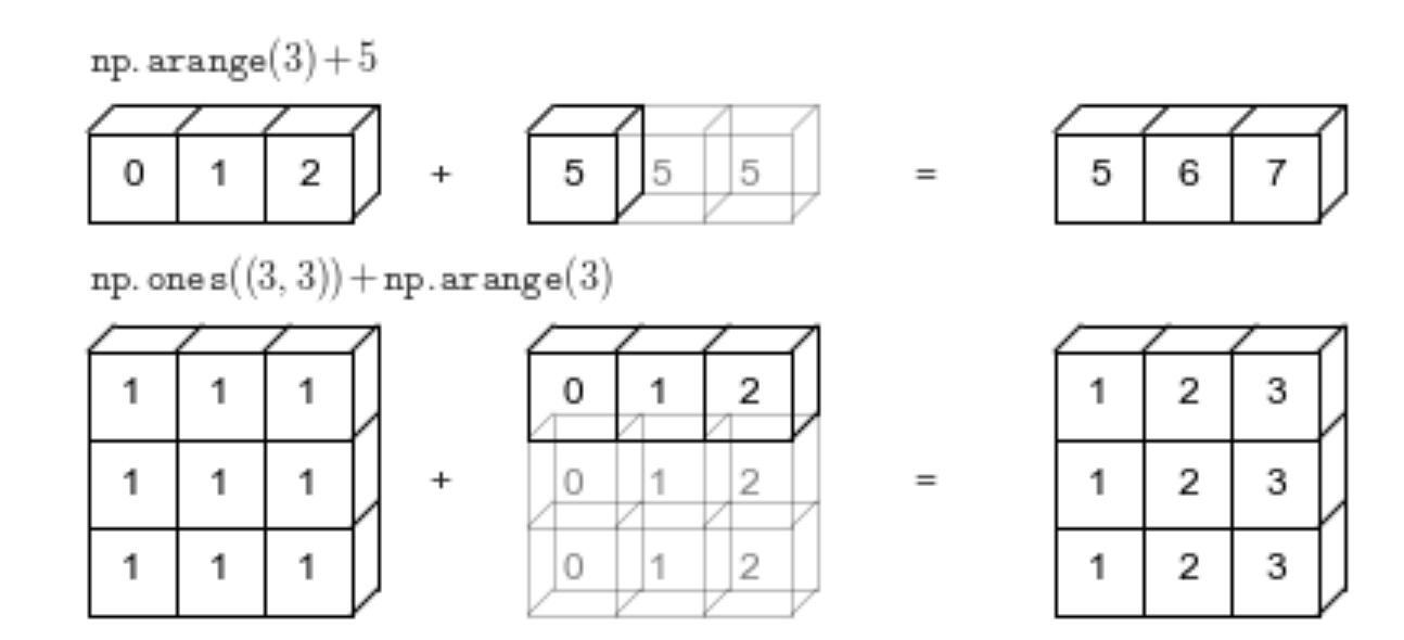
https://cdn.aibydoing.com/hands-on-ai/images/bd460f19c157886e5a89b411e86ff42b-0.jpg

如上所示： As shown above:

当一个一维向量和一个数字进行运算时，这个数字会被复制多份，直到和该向量的长度相等时，才进行计算。
當一個一維向量和一個數字進行運算時，這個數字會被複製多份，直到和該向量的長度相等時，才進行計算。
当一个二维数组和一个一维向量进行运算时，如果这个向量的长度和二维数组的某个维度相等，那么就会对该向量进行赋值，直到大小和二维数组相同。再进行运算。
當一個二維數組和一個一維向量進行運算時，如果這個向量的長度和二維數組的某個維度相等，那麼就會對該向量進行賦值，直到大小和二維數組相同。再進行運算。

在我们编写代码时，NumPy 会自动使用这种机制：
在我們編寫代碼時，NumPy 會自動使用這種機制：

                          a = np.array([[1, 2, 3], [4, 5, 6]])
b = np.array([[1, 2, 3]])
a+b

                        

array([[2, 4, 6],
       [5, 7, 9]])

值得注意的是，并不是所有大小不同的矩阵相加都可以进行广播。如果两个数组的尺寸在任何维度都不相同，且都不等于 1，那么就无法进行广播。NumPy 就会返回 operands could not be broadcast together with shapes 的错误。
It is worth noting that not all matrices of different sizes can be broadcasted. If the dimensions of the two arrays are not the same in any dimension and are not equal to 1, then broadcasting cannot be performed. NumPy will return an error of operands could not be broadcast together with shapes .

                          # 两个数组的尺寸在任何维度都不相同，且都不等于 1
a_ = np.array([[1, 2, 3], [4, 5, 6]])
b_ = np.array([[1, 2]])
a_+b_

                        

                          ---------------------------------------------------------------------------
ValueError                                Traceback (most recent call last)
Cell In[7], line 4
      2 a_ = np.array([[1, 2, 3], [4, 5, 6]])
      3 b_ = np.array([[1, 2]])
----> 4 a_+b_

ValueError: operands could not be broadcast together with shapes (2,3) (1,2) 

                        

88.10. 矩阵的性质# 88.10. 矩陣的性質 #

88.11. 矩阵的转置# 88.11. 矩陣的轉置 #

将矩阵的行列互换得到的新矩阵称为转置矩阵，记作 $A^{T}$ 。例子如下：
The new matrix obtained by interchanging the rows and columns of a matrix is called the transpose matrix, denoted as $A^{T}$ . An example is as follows:

\begin{array}{r} A = (\begin{array}{l} A_{1, 1} & A_{1, 2} \\ A_{2, 1} & A_{2, 2} \\ A_{3, 1} & A_{3, 2} \end{array}) \Rightarrow A^{T} = (\begin{array}{l} A_{1, 1} & A_{2, 1} & A_{3, 1} \\ A_{1, 2} & A_{2, 2} & A_{3, 2} \end{array}) \end{array}

如上所示，矩阵的转置就是把原矩阵的第 1 行的向量，变成了 1 列的向量。把原矩阵的第 2 行的向量，变成了 2 列的向量，直到所有的行向量变为列向量为止。
如上所示，矩陣的轉置就是把原矩陣的第 1 行的向量，變成了 1 列的向量。把原矩陣的第 2 行的向量，變成了 2 列的向量，直到所有的行向量變為列向量為止。

当然，如果使用 NumPy 来实现它的话是非常简单的，我们只需要在变量后面加上 .T 即可。如下：
當然，如果使用 NumPy 來實現它的話是非常簡單的，我們只需要在變量後面加上 .T 即可。如下：

                          print("a:")
print(a)
print("a 的转置矩阵:")
print(a.T)

                        

a:
[[1 2 3]
 [4 5 6]]
a 的转置矩阵:
[[1 4]
 [2 5]
 [3 6]]

88.12. 单位矩阵# 88.12. 單位矩陣 #

单位矩阵：n 阶单位矩阵，是一个 $n \times n$ 的方形矩阵（即行数和列数相同的矩阵），其主对角线元素为 1，其余元素为 0。单位矩阵一般用 $I_{n}$ 表示。形式如下：
Identity matrix: An n-order identity matrix is a square matrix (i.e., a matrix with the same number of rows and columns) with 1s on its main diagonal and 0s elsewhere. The identity matrix is generally denoted by I. It is represented as follows:

\begin{array}{r} I_{1} = [\begin{array}{l} 1 \end{array}], I_{2} = [\begin{array}{l} 1 & 0 \\ 0 & 1 \end{array}], I_{3} = [\begin{array}{l} 1 & 0 & 0 \\ 0 & 1 & 0 \\ 0 & 0 & 1 \end{array}] . . . . . . . . . . . . . I_{n} = [\begin{array}{l} 1 & 0 & \dots & 0 \\ 0 & 1 & \dots & 0 \\ ⋮ & ⋮ & ⋱ & ⋮ \\ 0 & 0 & \dots & 1 \end{array}] \end{array}

可以直接用 np.identity() 来定义一个单位矩阵：
You can directly use np.identity() to define an identity matrix:

                          # 传入大小 n
np.identity(4)

array([[1., 0., 0., 0.],
       [0., 1., 0., 0.],
       [0., 0., 1., 0.],
       [0., 0., 0., 1.]])

88.13. 矩阵的逆# 88.13. Inverse of a Matrix

方阵 $A$ 的逆矩阵记作 $A^{- 1}$ ,且该矩阵满足如下条件：
The inverse matrix of matrix $A$ is denoted as $A^{- 1}$ , and this matrix satisfies the following conditions:

A^{- 1} A = I_{n}

也就是说，如果一个矩阵和 $A$ 的乘积（传统乘积）为一个单位矩阵，那么这个矩阵就是 $A$ 的逆矩阵。
In other words, if the product (traditional product) of a matrix and $A$ is an identity matrix, then this matrix is the inverse matrix of $A$ .

关于 $A$ 的逆矩阵在数学上的具体求法，这里就不做阐述了。我们直接使用 NumPy 对其进行求取：
Regarding the specific method of finding the inverse matrix of $A$ in mathematics, it will not be elaborated here. We will directly use NumPy to obtain it:

                          a = np.array([[1, 2], [3, 4]])
# 通过 np.linalg.inv() 求取逆矩阵
print(np.linalg.inv(a))
print("=================")
# 矩阵对象可以通过 ‘.I’ 属性，更方便的求逆
A = np.matrix(a)
print(A.I)

                        

[[-2.   1. ]
 [ 1.5 -0.5]]
=================
[[-2.   1. ]
 [ 1.5 -0.5]]

如上，我们提供了两种逆矩阵的求取方式。 As mentioned above, we have provided two methods for finding the inverse matrix.

我们一般把上面这种可逆的矩阵称之为非奇异矩阵，把那些不可逆的矩阵称之为奇异矩阵。而区分矩阵是否可逆的方法有很多中，其中用的最多的就是判断该矩阵的行列式。
We generally refer to the reversible matrix mentioned above as a non-singular matrix, and those irreversible matrices as singular matrices. There are many methods to distinguish whether a matrix is reversible, among which the most commonly used is to determine the determinant of the matrix.

如果该矩阵为一个方阵且方阵的行列式不等于 0 ，则表示该矩阵可逆。
If the matrix is a square matrix and its determinant is not equal to 0, it means the matrix is invertible.
否则，不可逆（即为奇异矩阵）。 Otherwise, it is irreversible (i.e., a singular matrix).

88.14. 矩阵的行列式# 88.14. Determinant of a Matrix

行列式是方阵(即行数和列数相等的矩阵)才有的一种特征，记作 $d e t (A)$ ，也记作 $| A |$ 。它的计算公式较为复杂，是很多同学上学时的噩梦。当然作为一个程序员来说，我们不需要对该行列式的具体计算步骤了然于心，我们只需要知道如何求它用它即可。
The determinant is a characteristic of a square matrix (i.e., a matrix with an equal number of rows and columns), denoted as $d e t (A)$ or $| A |$ . Its calculation formula is quite complex and is a nightmare for many students during their school years. Of course, as a programmer, we do not need to be thoroughly familiar with the specific calculation steps of the determinant; we only need to know how to find and use it.

我们可以使用 np.linalg.det() 对行列式进行求取：
We can use np.linalg.det() to calculate the determinant:

                          a = np.array([[1, 2], [3, 4]])
b = np.array([[1, 2], [2, 4]])
print("a的行列式为", np.linalg.det(a))
print("b的行列式为", np.linalg.det(b))

                        

a的行列式为 -2.0000000000000004
b的行列式为 0.0

从上面的结果可知，a 矩阵的行列式不为 0 ，为可逆矩阵。而 b 矩阵的行列式为 0 ，为不可逆矩阵。你可以尝试用 np.linalg.inv() 方法求取一下 b 的逆矩阵，观察程序是否报错。
From the above results, it can be seen that the determinant of matrix a is not 0, making it an invertible matrix. However, the determinant of matrix b is 0, making it a non-invertible matrix. You can try using the np.linalg.inv() method to find the inverse of b and observe whether the program reports an error.

88.15. 范数# 88.15. Norms #

在机器学习中我们经常需要使用到范数来衡量向量的大小。范数的形式有很多种，而机器学习中经常使用的是 L2 范数，又称做欧几里得范数。该范数的计算公式如下：
In machine learning, we often need to use norms to measure the size of vectors. There are many forms of norms, and the one frequently used in machine learning is the L2 norm, also known as the Euclidean norm. The calculation formula for this norm is as follows:

| | x | |_{2} = \sqrt{\sum_{i = 1}^{N} x_{i}^{2}}

根据公式，我们不难发现向量的 L2 范数其实就是绝对值的平方和再开方。
According to the formula, it is not difficult to find that the L2 norm of a vector is actually the square root of the sum of the squares of its absolute values.

L2 范数除来被应用于传统机器学习中，如岭回归、贝叶斯推断等，还被广泛应用于深度学习中。如利用 L2 范数进行的正则化，可以很好的缓解神经网络权重的衰减，提高模型的泛化能力。
The L2 norm is not only applied in traditional machine learning, such as ridge regression and Bayesian inference, but also widely used in deep learning. For example, regularization using the L2 norm can effectively alleviate the decay of neural network weights and improve the generalization ability of the model.

我们可以通过 np.linalg.norm() 对 L2 范数进行计算：
We can calculate the L2 norm through np.linalg.norm() :

                          print("按列向量计算 a 的范数", np.linalg.norm(a, axis=0))  # 按列向量计算范数
print("按行向量计算 a 的范数", np.linalg.norm(a, axis=1))  # 按行向量计算范数
print("计算矩阵 a 的范数", np.linalg.norm(a))  # 按列向量计算范数

                        

按列向量计算 a 的范数 [3.16227766 4.47213595]
按行向量计算 a 的范数 [2.23606798 5.        ]
计算矩阵 a 的范数 5.477225575051661

88.16. 矩阵的迹# 88.16. Trace of the Matrix

矩阵的迹即为矩阵的对角元素（即对角线上的所有元素）之和，记作 $T r (A)$ 。计算公式如下：
The trace of a matrix is the sum of its diagonal elements (i.e., all the elements on the diagonal), denoted as $T r (A)$ . The formula is as follows:

T r (A) = A_{11} + A_{22} + A_{33} . . . . . = \sum_{i} A_{i i}

我们可以使用 np.trace()，快速的求取一个矩阵的迹，如下：
We can use np.trace() to quickly find the trace of a matrix, as follows:

                          print("a_00：", a[0][0])
print("a_11：", a[1][1])
print("Tr(a)：", np.trace(a))

                        

a_00： 1
a_11： 4
Tr(a)： 5

88.17. 特殊的矩阵# 88.17. Special Matrices

对角矩阵：只在主对角线上含有非零元素，其他位置都为零的矩阵。其实这和上面的单位矩阵很像，只是单位矩阵的对角线上必须为 1 ，对角矩阵的对角线上可以为非零的任意值。因此对角矩阵 $d i a g (x)$ 的形式如下：
Diagonal matrix: A matrix that contains non-zero elements only on the main diagonal, with all other positions being zero. In fact, this is very similar to the identity matrix, except that the diagonal of the identity matrix must be 1, while the diagonal of a diagonal matrix can be any non-zero value. Therefore, the form of the diagonal matrix $d i a g (x)$ is as follows:

\begin{array}{r} d i a g (x) = [\begin{array}{l} x_{1} & 0 & \dots & 0 \\ 0 & x_{2} & \dots & 0 \\ ⋮ & ⋮ & ⋱ & ⋮ \\ 0 & 0 & \dots & x_{n} \end{array}] \end{array}

可以直接用 np.diag() 来定义一个对角矩阵：
You can directly use np.diag() to define a diagonal matrix:

                          # 函数传入的是对角线上的值
x = np.diag((1, 2, 3, 4))
x

                        

array([[1, 0, 0, 0],
       [0, 2, 0, 0],
       [0, 0, 3, 0],
       [0, 0, 0, 4]])

有趣的是，该函数除了创造对角矩阵，还能从对角矩阵中提取出对角线上的值：
Interestingly, this function not only creates a diagonal matrix but also extracts the values on the diagonal from a diagonal matrix:

                          np.diag(x)

                        

array([1, 2, 3, 4])

对称矩阵：如果矩阵 $A$ 的转置和矩阵 $A$ 相同，则矩阵 $A$ 就是对称矩阵。换句话说，若矩阵 $A$ 满足 $A_{i j} = A_{j i}$ ，其中 $i$ ， $j$ 为任意值，则 $A$ 为对称矩阵。
Symmetric Matrix: If the transpose of matrix $A$ is the same as matrix $A$ , then matrix $A$ is a symmetric matrix. In other words, if matrix $A$ satisfies $A_{i j} = A_{j i}$ , where $i$ and $j$ are arbitrary values, then $A$ is a symmetric matrix.

因为转置相同，所以矩阵 $A$ 的行数必须等于列数，即矩阵必定是方阵。因为对称，所以上三角（对角线上面的三角形内容）和下三角的内容必定对称。如下所示：
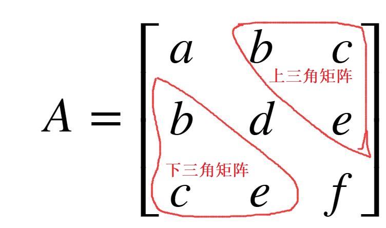
Because the transpose is the same, the number of rows of the matrix $A$ must be equal to the number of columns, that is, the matrix must be a square matrix. Because of symmetry, the contents of the upper triangle (the triangular content above the diagonal) and the lower triangle must be symmetrical. As shown below:

https://cdn.aibydoing.com/hands-on-ai/images/b268a1a25089cad4dc781524b699fe45-0.jpg

从上面的实例可以看出，该矩阵的沿着对角线对称，矩阵上三角的内容等于矩阵下三角的内容。

不过，NumPy 中没有现成的库来直接创建对称矩阵，对称矩阵的创建步骤如下：

首先让我们初始化一个 $5 \times 5$ 的矩阵：

                          # 随机初始化 25 个数，然后将这一组数转换为 5*5 的矩阵
x = np.random.randn(25).reshape(5, 5)
x

                        

array([[-1.76147734, -0.86482382,  0.62757387, -1.30881442, -2.1407301 ],
       [-1.95812775, -0.02321958,  0.6240782 , -0.48150296,  0.90741739],
       [-0.03717522, -1.26331227,  1.10608778,  0.39242673, -1.16064422],
       [ 1.1341177 , -1.81348565,  0.92502167,  1.95435312, -0.05584964],
       [-1.54326738,  1.16051111,  1.1648892 , -2.28413737,  0.50776626]])

然后利用 triu()函数取出矩阵 x 的上三角矩阵：

                          cov_up = np.triu(x)
cov_up

array([[-1.76147734, -0.86482382,  0.62757387, -1.30881442, -2.1407301 ],
       [ 0.        , -0.02321958,  0.6240782 , -0.48150296,  0.90741739],
       [ 0.        ,  0.        ,  1.10608778,  0.39242673, -1.16064422],
       [ 0.        ,  0.        ,  0.        ,  1.95435312, -0.05584964],
       [ 0.        ,  0.        ,  0.        ,  0.        ,  0.50776626]])

接下来，我们我们需要获得将上三角矩阵转置，即得到与之对称的下三角矩阵，如下：

                          cov_down = cov_up.T
cov_down

array([[-1.76147734,  0.        ,  0.        ,  0.        ,  0.        ],
       [-0.86482382, -0.02321958,  0.        ,  0.        ,  0.        ],
       [ 0.62757387,  0.6240782 ,  1.10608778,  0.        ,  0.        ],
       [-1.30881442, -0.48150296,  0.39242673,  1.95435312,  0.        ],
       [-2.1407301 ,  0.90741739, -1.16064422, -0.05584964,  0.50776626]])

然后，我们将上三角矩阵和下三角矩阵相加即可：

                          cov_up_down = cov_up+cov_down
cov_up_down

array([[-3.52295468, -0.86482382,  0.62757387, -1.30881442, -2.1407301 ],
       [-0.86482382, -0.04643916,  0.6240782 , -0.48150296,  0.90741739],
       [ 0.62757387,  0.6240782 ,  2.21217556,  0.39242673, -1.16064422],
       [-1.30881442, -0.48150296,  0.39242673,  3.90870625, -0.05584964],
       [-2.1407301 ,  0.90741739, -1.16064422, -0.05584964,  1.01553252]])

细心的你可能已经发现，尽管这样可以得到一个对称矩阵，但是我们将对角线的值加了两次（上三角矩阵和下三角矩阵中的对角线的值都存在）。因此，最后，我们需要将得到的 cov_up_down 减去一个对角线的值。

首先，让我们来初始化只有对角线元素有值的对角矩阵：

                          # 获得对角线的值
d = np.diag(x)
# 获得对角矩阵
dia = np.diag(d)
dia

                        

array([[-1.76147734,  0.        ,  0.        ,  0.        ,  0.        ],
       [ 0.        , -0.02321958,  0.        ,  0.        ,  0.        ],
       [ 0.        ,  0.        ,  1.10608778,  0.        ,  0.        ],
       [ 0.        ,  0.        ,  0.        ,  1.95435312,  0.        ],
       [ 0.        ,  0.        ,  0.        ,  0.        ,  0.50776626]])

最后减去一个对角矩阵，得到最后的对称矩阵：

                          x = cov_up_down-dia
x

array([[-1.76147734, -0.86482382,  0.62757387, -1.30881442, -2.1407301 ],
       [-0.86482382, -0.02321958,  0.6240782 , -0.48150296,  0.90741739],
       [ 0.62757387,  0.6240782 ,  1.10608778,  0.39242673, -1.16064422],
       [-1.30881442, -0.48150296,  0.39242673,  1.95435312, -0.05584964],
       [-2.1407301 ,  0.90741739, -1.16064422, -0.05584964,  0.50776626]])

我们可以利用矩阵的转置等于矩阵本身来测试一下 x 是否为对称矩阵：

                          x == x.T

                        

array([[ True,  True,  True,  True,  True],
       [ True,  True,  True,  True,  True],
       [ True,  True,  True,  True,  True],
       [ True,  True,  True,  True,  True],
       [ True,  True,  True,  True,  True]])

正交矩阵：当方阵 $A$ 满足 $A^{T} A = A A^{T} = I$ 时， $A$ 被叫做正交矩阵。

根据逆矩阵的定义可知，若矩阵可逆，则有 $A^{- 1} A = I$ 。因此结合上面两个式子，若矩阵 $A$ 既为逆矩阵又为正交矩阵，则有：

A^{- 1} = A^{T}

88.18. 矩阵的分解#

88.19. 特征值与特征分解#

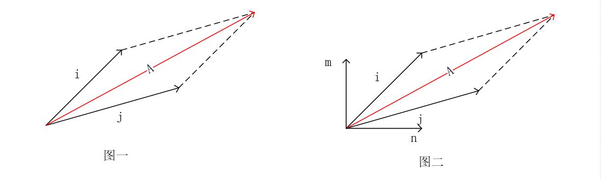
还记得我们高中时学过的力的合成吗？力 $\vec{j}$ 和力 $\vec{i}$ 可以通过叠加得到力 $\vec{A}$ ，记作 $（ \vec{i}, \vec{j} ）$ ,如下图一所示：

https://cdn.aibydoing.com/hands-on-ai/images/3afce0e479adeff121dc03dbed7328ea-0.jpg

从图 1 可以看到，当以 $i, j$ 为坐标轴时，A 可以被表示为 $1 \vec{i} + 1 \vec{j}$ 。换句话说，在 $i, j$ 的坐标空间中，A 的坐标为 $(1 i, 1 j)$ 。

但是，显然利用 $i$ ， $j$ 来表示的合成力 $A$ 并不能很好的展现物体的作用效果（即该力作用下的物体会向上走多少，向右走多少）。因此，我们常常会再做一次变换，将力分解到横向和竖直两个方向，即将力 $A$ 转换到图二所示的 $\vec{m}$ 和 $\vec{n}$ 坐标空间中，那么此时 $A$ 的坐标就不再是 $(1 i, 1 j)$ 了，而是 $(λ_{1} m, λ_{2} n)$ 。

而特征分解的原理和力的分解类似，也就是将一个方阵 $A$ 转换为新的空间下的矩阵的过程。其中新空间下的坐标轴向量被称之为特征向量（记作 $v$ ），而矩阵 $A$ 与特征向量的倍数称之为特征值，记作 $λ$ (即上面的 $λ_{1}, λ_{2} . . .$ 的集合)。

我们可以用 $λ v$ 来表示方阵 $A$ 在新空间下的坐标，同样，根据矩阵乘法的物理性质，我们也可以用 $A \cdot v$ 来表示原方阵 $A$ 转换到特征向量为 $v$ 的新空间的过程。

因此，矩阵 $A$ 和它的特征向量、特征值必定满足下列等式：

A v = λ v

假设方阵 $A$ 的特征向量集合为 $V = v_{1}, v_{2}, . . ., v_{n}$ ，特征值的集合为 $λ = λ_{1}, λ_{2}, . . ., λ_{n}$ 。根据上列等式，我们可以得到 $A$ 的关系式如下（等号两边同时右乘 $V^{- 1}$ ）：

A = V d i a g (λ) V^{- 1}

已知 $A$ ，需要求解上面的 $V$ 和 $λ$ 的算法是非常复杂的，需要使用到上面的正交矩阵、对角矩阵等相关知识，可参照这篇文章。

这里，我们直接使用 vals,vecs = np.linalg.eig(x) 函数来完成特征分解，求解 $V$ 和 $λ$ 的具体值。该函数主要有两个返回值：

第一个返回变量为分解得到的特征值。
第二个返回变量为每个特征值所对应的特征向量。

                          a = np.array([[1, 2, 3], [5, 8, 7], [1, 1, 1]])
e_vals, e_vecs = np.linalg.eig(a)
print("特征值为：", e_vals)
print("特征向量为：\n", e_vecs)

                        

特征值为： [10.254515   -0.76464793  0.51013292]
特征向量为：
 [[-0.24970571 -0.89654947  0.54032982]
 [-0.95946634  0.19306928 -0.73818337]
 [-0.13065753  0.39865186  0.40389232]]

如上所示，矩阵 $a$ 被分解成了特征值 $e_v a l s$ 和特征向量 $e_v e c s$ ，一个特征向量对应一个特征值。

那么得到的特征值和特征向量在机器学习中到底有什么用呢？

从上面的学习中，我们可以很容易的得到下面这个结论：特征分解其实就是将原矩阵中的向量方向和距离进行了分离。我么可以得到每个特征向量上的特征值，进而比较每组向量（特征向量+特征值）对原矩阵内容的贡献程度。

就拿上面的测试代码进行举例，我们已经得到了 $a$ 矩阵的三个特征值和所对应的特征向量。现在让我们来计算一下，每个特征值占总特征值的百分比进而估算每个特征向量对原矩阵的贡献程度（这里的特征值都需要先进行绝对值，再求和。因为这里的正负号，表示的只是方向而已）。

                          pro = abs(e_vals)/np.sum(abs(e_vals))
pro

array([0.88943116, 0.06632217, 0.04424667])

从上面可以看出，第一组（特征向量+特征值）对原矩阵内容的贡献程度能够达到 89%，而其他两组只有 6.6% 和 4.4%。当然，由于这里的矩阵只是一个 $3 \times 3$ 的矩阵，我们很难看出特征分解的巨大作用。

但是请想象一下，如果这个矩阵为 $1000 \times 1000$ 的矩阵，当把它特征分解成特征值+特征性向量时，有两组特征值+特征向量对原矩阵的内容贡献程度之和就有 89% ，而其他 998 组的贡献之和却只有 11% 。那么，我们是不是就可以把那些对原矩阵内容贡献程度较小的特征值+特征向量给删除掉呢？

也就是说，我们可以用两组特征值+特征向量来表示这个 $1000 \times 1000$ 矩阵的 89% 的内容。这就是数据降维，即在保存原数据大部分内容的情况下，缩小数据量，减少数据特征的过程。

当然也并不是说所有矩阵都可以进行特征分解，只有在矩阵为可逆的方阵时，特征分解才有效。

而我们在日常生活中接触到的数据，很难是一个完完整整的方阵。有可能只有 100 个特征，每个特征却有 10000 条数据。因此，接下来我们将会介绍一种更加普适的矩阵分解的方法：奇异值分解。

88.20. 奇异值分解#

奇异值分解 (SVD) 也是一种矩阵分解方法，该方法可以将矩阵分解为奇异向量和奇异值。奇异值分解不仅仅是一个数学问题，在工程领域中的应用也非常广泛。比如现行的一些推荐系统中。

我们对任意实数矩阵 $A$ 的奇异分解过程，可以表示为：

A = U D V^{T}

其中 $D$ 为对角矩阵，而它对角线上的元素就被称之为奇异值。矩阵 $U$ 的列向量被称之为「左奇异向量」，矩阵 $V$ 的列向量被称之为「右奇异向量」。当我们需要对矩阵的行数进行压缩时，我们使用到的组合就是：左奇异向量 + 奇异值。当我们是对矩阵的列数进行压缩降维时，我们使用到的就是：右奇异向量 + 奇异值。

同样，已知 $A$ ，求取 $U$ 、 $D$ 、 $V$ 的数学推导公式非常复杂，这里我们直接使用 NumPy 对其进行接求解。

我们使用 np.linalg.svd(a) 函数对矩阵 $A$ 进行奇异值分解，得到下面三个返回值：

第一个返回值：矩阵 $A$ 的左奇异向量 $U$ 。
第二个返回值：对角矩阵 $D$ 的对角线上的值（对角矩阵除了对角线，其他位置的值都为 0 ）。
第三个返回值，矩阵 $A$ 的右奇异向量 $V$ 的转置 $V^{T}$ 。

                          a = np.array([[1, 2, 3, 4], [5, 8, 6, 7], [1, 1, 1, 2]])
u, s, vh = np.linalg.svd(a)  # vh 表示 v 的转置
print(u.shape, s.shape, vh.shape)

                        

(3, 3) (3,) (4, 4)

现在我们可以验证一下，利用 NumPy 求出来的奇异值和奇异向量是否真正满足奇异分解的公式，是否能够全权代表原矩阵的内容。

首先，让我们先把 $s$ 转为对角矩阵 $D$ 。为了能够左乘 $U$ 和右乘 $V^{T}$ ，因此生成的对角矩阵 $D$ 的大小必须为 $3 \times 4$ :

                          # 初始化 3×4 全为 0 的矩阵
D = np.zeros((3, 4))
# np.diag(s) 只能生成 3×3 的矩阵
D[:3, :3] = np.diag(s)
D

                        

array([[14.37981705,  0.        ,  0.        ,  0.        ],
       [ 0.        ,  1.97748535,  0.        ,  0.        ],
       [ 0.        ,  0.        ,  0.55714755,  0.        ]])

最后，将它们相乘，观察得到的结果是否和 $A$ 一致：

                          # 但传入的两个变量之间的差距在 0.00001 以内时，返回true
np.allclose(a, np.dot(u, np.dot(D, vh)))

True

至此，我学习完了机器学习中会用到的线性代数知识。接下来，让我们利用已学到的线性代数知识来实现 PCA 算法，并完成鸢尾花数据集的可视化工作。

88.21. 鸢尾花数据集的可视化#

88.22. 数据集的简介#

鸢尾花数据集是机器学习中最常用的数据集之一。该数据集合包含了三类鸢尾花，一共 150 条数据。每条数据记录了一朵花的花萼长度、花萼宽度、花瓣长度以及花瓣宽度等四个特征，并且标注了该花属于哪一种鸢尾花。

让我们利用 scikit-learn 库来加载该数据集合：

                          from sklearn import datasets
iris = datasets.load_iris()
# 加载特征
iris_data = iris['data']
# 加载标签
iris_label = iris['target']
print(iris_data.shape)
print(iris_label.shape)

                        

(150, 4)
(150,)

其中 iris_data 变量中保存了 150 朵花具有的 4 种特征，iris_label 代表着这 150 朵花各自的类型。

接下来，我们想要把这些样本点画在坐标系中，观察数据点和花的种类的关系。但是，由于该花有四个特征，而我们最多在三维空间中画图。因此，我们需要对原数据集合进行降维，使其维度减小到 2 或 3，这样我们就能够进行可视化了。而这里，我们使用到的降维方法就是主成分分析法（PCA）。

88.23. 主成分分析法#

主成分分析（PCA）是一种用于数据压缩的机器学习算法。该算法可以将线性相关性的高维变量分解成线性无关的低维变量。新的低维变量可以保留原始数据的大部分信息，进而达到降维的效果。

主成分分析法的主要实现方式有两种，一种基于特征值分解，而另外一种基于奇异值分解。

基于奇异值分解 的具体步骤如下：

对样本数据进行去中心化处理，并得到数据 $x$ 。
对 $x$ 进行 SVD 奇异分解得到 $u, s, v$ 。
取 $v$ 的前 $d$ 个右奇异向量，记作 $v [0 : d]$ 。
$x \cdot v [0 : d]$ 就是低维空间的数据（也可以使用奇异值乘以奇异向量得到该数据）。

这里的去中心化处理就是让每个元素值减去自己所在维度的均值。这样可以使输入数据的各个维度的均值为 0 （由于存在小数，因此可能会无限接近于0，但不等于0 ），进而增加数据的鲁棒性。如下：

                          data_cen = iris_data - np.mean(iris_data, axis=0)  # 样本中心化处理
# 去中心化后的矩阵的每个维度的平均值无限接近于 0
np.mean(data_cen, axis=0)

                        

array([-1.12502600e-15, -7.60872846e-16, -2.55203266e-15, -4.48530102e-16])

接下来，让我们根据上面步骤，完成基于 SVD 的 PCA 函数：

                          def pca_svd(data):
    # 进行svd 分解
    u, s, v = np.linalg.svd(data)
    # 这里选取前两个特征v[0:2]
    # 然后计算低维空间数据
    pc_svd = np.dot(data, v[:, 0:2])
    return pc_svd


pc_svd = pca_svd(data_cen)
pc_svd

                        

array([[-2.24698392,  1.46899397],
       [-1.99096685,  1.85097919],
       [-2.25276491,  1.78164249],
       [-2.10683872,  1.74352871],
       [-2.34878146,  1.40443007],
       [-2.16349706,  0.90825477],
       [-2.33046962,  1.55229906],
       [-2.15926072,  1.49067128],
       [-2.10600127,  1.96625659],
       [-2.02997146,  1.75014427],
       [-2.21168271,  1.23781384],
       [-2.17333505,  1.4477847 ],
       [-2.05865423,  1.89140375],
       [-2.41395648,  2.11303825],
       [-2.43871366,  1.16432965],
       [-2.49978144,  0.63739946],
       [-2.396309  ,  1.1474191 ],
       [-2.2154352 ,  1.43702166],
       [-2.02097092,  0.98788647],
       [-2.35420885,  1.15818214],
       [-1.89830011,  1.33728011],
       [-2.25700125,  1.19922598],
       [-2.72614803,  1.67740341],
       [-1.84641105,  1.33973607],
       [-1.99872609,  1.26841145],
       [-1.83842222,  1.72294477],
       [-2.03796029,  1.36693557],
       [-2.15264228,  1.40075063],
       [-2.14518638,  1.53355786],
       [-2.07815596,  1.60226924],
       [-1.97635842,  1.66683313],
       [-1.95160864,  1.39291765],
       [-2.57814426,  0.99462608],
       [-2.56204142,  0.92407196],
       [-1.99842274,  1.71817196],
       [-2.20255192,  1.81607681],
       [-2.16063227,  1.49497604],
       [-2.41646883,  1.44485464],
       [-2.22986313,  1.95303153],
       [-2.12312206,  1.48221903],
       [-2.30977685,  1.50526499],
       [-1.70256362,  2.42371997],
       [-2.36118089,  1.80699924],
       [-2.04052173,  1.22997481],
       [-2.08984819,  0.8870455 ],
       [-1.99555679,  1.82745913],
       [-2.32755458,  1.13036337],
       [-2.23070058,  1.73030365],
       [-2.24782137,  1.24626609],
       [-2.15180483,  1.6234785 ],
       [ 0.93591038, -0.82932384],
       [ 0.63422117, -0.69100048],
       [ 1.11338528, -0.89940993],
       [ 0.54579077,  0.40511511],
       [ 0.99119832, -0.46717924],
       [ 0.58078863, -0.27582553],
       [ 0.68037832, -0.90711885],
       [-0.23876712,  0.89726699],
       [ 0.89858067, -0.48470301],
       [ 0.14808502,  0.16622606],
       [ 0.17641302,  1.06129714],
       [ 0.41023667, -0.32333369],
       [ 0.69749678,  0.53178693],
       [ 0.80763908, -0.53420515],
       [-0.04483578,  0.19773033],
       [ 0.71854432, -0.5515777 ],
       [ 0.47642965, -0.47735018],
       [ 0.35512806,  0.12381963],
       [ 1.21853262,  0.05606546],
       [ 0.32931125,  0.37436628],
       [ 0.72278299, -0.9240294 ],
       [ 0.43432834, -0.01067912],
       [ 1.29050659, -0.41059956],
       [ 0.81020051, -0.39724439],
       [ 0.65169439, -0.28842526],
       [ 0.74806454, -0.4701093 ],
       [ 1.18447155, -0.58014585],
       [ 1.22806727, -0.93322498],
       [ 0.68664317, -0.43814304],
       [ 0.03543037,  0.56403452],
       [ 0.30062848,  0.51562575],
       [ 0.21087678,  0.60738915],
       [ 0.30181953,  0.17945718],
       [ 1.19872755, -0.68282957],
       [ 0.40415233, -0.46044568],
       [ 0.3898975 , -0.83519607],
       [ 0.924702  , -0.76292326],
       [ 1.06771198,  0.09833277],
       [ 0.18052027, -0.17424123],
       [ 0.41447301,  0.25908282],
       [ 0.55007736, -0.02112534],
       [ 0.68377721, -0.54743021],
       [ 0.42568139,  0.19268224],
       [-0.13696958,  0.96183088],
       [ 0.43569989, -0.01498388],
       [ 0.2433132 , -0.21051225],
       [ 0.34052079, -0.16946842],
       [ 0.57941707, -0.27152076],
       [-0.37520891,  0.95474728],
       [ 0.34797669, -0.03666119],
       [ 1.7209556 , -1.97215372],
       [ 1.22109639, -0.76184199],
       [ 2.02264365, -1.63304298],
       [ 1.52993814, -1.21711864],
       [ 1.77915743, -1.5545107 ],
       [ 2.61075784, -2.09384182],
       [ 0.61485086, -0.11704833],
       [ 2.29874562, -1.72017874],
       [ 2.05353425, -1.07844524],
       [ 1.90742989, -2.3270635 ],
       [ 1.17732134, -1.21806078],
       [ 1.55433431, -0.93213767],
       [ 1.68141573, -1.36852189],
       [ 1.28962122, -0.57953868],
       [ 1.31318111, -0.99471969],
       [ 1.35223481, -1.42510763],
       [ 1.47835359, -1.24724821],
       [ 2.21137718, -2.77818661],
       [ 3.1472384 , -2.05354736],
       [ 1.43727023, -0.22598545],
       [ 1.76574004, -1.70653322],
       [ 0.99830294, -0.73034378],
       [ 2.80486852, -1.98408055],
       [ 1.253835  , -0.65254877],
       [ 1.56470641, -1.69870024],
       [ 1.89102138, -1.75140167],
       [ 1.09383447, -0.65732158],
       [ 0.98458105, -0.8546927 ],
       [ 1.72638183, -1.24847168],
       [ 1.84283572, -1.42184259],
       [ 2.31568591, -1.56800499],
       [ 2.04594811, -2.55177324],
       [ 1.75793055, -1.28044399],
       [ 1.20993593, -0.74923015],
       [ 1.52844257, -0.85327647],
       [ 2.41897901, -1.86728327],
       [ 1.39093607, -1.77403322],
       [ 1.37655606, -1.3118121 ],
       [ 0.8902394 , -0.78644937],
       [ 1.59369253, -1.3901992 ],
       [ 1.73246734, -1.5887938 ],
       [ 1.48218101, -1.27477057],
       [ 1.22109639, -0.76184199],
       [ 1.84600735, -1.81766313],
       [ 1.69090129, -1.82658948],
       [ 1.53376555, -1.24464101],
       [ 1.47490445, -0.59827988],
       [ 1.36684208, -1.13181958],
       [ 1.20684272, -1.61402649],
       [ 1.0287097 , -0.95737037]])

如上所示，我们已经对原数据进行了降维，得到了两列新的数据。这两列新的数据可以表示原数据的大部分内容。现在，我们就可以用一个二维的图像，来展示这 150 条数据的分布情况了。

                          import matplotlib.pyplot as plt
%matplotlib inline
plt.scatter(pc_svd[:, 0], pc_svd[:, 1], c=iris_label)
plt.show()

                        

../_images/01f481204cdaf25d22d48ba761f50815f6eebd5c0114dd373b496498f69ba0f6.png

上图很直观的展示出了，这三种鸢尾花的分布情况。当然值得注意的是，这两列新的数据和原来的任何一列数据都不同。这两列数据是通过 SVD 从原来四列数据信息中，生成的两列新的数据。

基于特征值分解 的步骤和基于 SVD 的步骤类似，但是由于能够特征分解的矩阵只能为方阵。因此在进行特征分解之前，我们还需要对矩阵进行一次处理，得到该矩阵的协方差矩阵（任意矩阵的协方差矩阵必定为方阵）。具体步骤如下：

对原始数据集进行去中心化处理，得到数据集 X。
计算数据集 X 的协方差矩阵 $X X^{T}$ 。
对协方差矩阵 $X X^{T}$ 做特征分解。
取最大的 $d$ 个特征值所对应的特征向量。
矩阵 X 乘以这 $d$ 个特征向量，得到低维空间数据（当然也可以使用筛选后的特征值乘以特征向量得到低维空间数据）。

这里我们涉及到了一个新的概念，协方差矩阵。该矩阵的计算公式为 $X X^{T}$ 。假设原数据 X 的大小为 $m \times n$ ，则 $X^{T}$ 的大小为 $n \times m$ 。则协方差矩阵 $X X^{T}$ 的大小为 $m \times m$ ，即 $X X^{T}$ 为方阵。这样我们就可以进行特征分解了。当然关于协方差矩阵的更多知识点，我们会在后面的统计学中讲到。

根据上面的阐述，让我们来定义基于特征值分解的 PCA 函数，如下：

                          def pca_eig(data_cen):
    # 计算协方差矩阵,每行为一个样本
    cov_mat = np.cov(data_cen, rowvar=0)
    eigVals, eigVects = np.linalg.eig(cov_mat)
    # 对特征值进行排序
    eigValInd = np.argsort(eigVals)
    # 排序是从小到大排序，因此选择最后面两个
    eigValInd = eigValInd[:-3:-1]
    # 得到投影矩阵，即对原内容来说，最为关键特征向量
    redEigVects = eigVects[:, eigValInd]
    # 通过投影矩阵得到降维后的数据
    pc_eig = np.dot(data_cen, redEigVects)
    return pc_eig


pc_eig = pca_eig(data_cen)
pc_eig

                        

array([[-2.68412563, -0.31939725],
       [-2.71414169,  0.17700123],
       [-2.88899057,  0.14494943],
       [-2.74534286,  0.31829898],
       [-2.72871654, -0.32675451],
       [-2.28085963, -0.74133045],
       [-2.82053775,  0.08946138],
       [-2.62614497, -0.16338496],
       [-2.88638273,  0.57831175],
       [-2.6727558 ,  0.11377425],
       [-2.50694709, -0.6450689 ],
       [-2.61275523, -0.01472994],
       [-2.78610927,  0.235112  ],
       [-3.22380374,  0.51139459],
       [-2.64475039, -1.17876464],
       [-2.38603903, -1.33806233],
       [-2.62352788, -0.81067951],
       [-2.64829671, -0.31184914],
       [-2.19982032, -0.87283904],
       [-2.5879864 , -0.51356031],
       [-2.31025622, -0.39134594],
       [-2.54370523, -0.43299606],
       [-3.21593942, -0.13346807],
       [-2.30273318, -0.09870885],
       [-2.35575405,  0.03728186],
       [-2.50666891,  0.14601688],
       [-2.46882007, -0.13095149],
       [-2.56231991, -0.36771886],
       [-2.63953472, -0.31203998],
       [-2.63198939,  0.19696122],
       [-2.58739848,  0.20431849],
       [-2.4099325 , -0.41092426],
       [-2.64886233, -0.81336382],
       [-2.59873675, -1.09314576],
       [-2.63692688,  0.12132235],
       [-2.86624165, -0.06936447],
       [-2.62523805, -0.59937002],
       [-2.80068412, -0.26864374],
       [-2.98050204,  0.48795834],
       [-2.59000631, -0.22904384],
       [-2.77010243, -0.26352753],
       [-2.84936871,  0.94096057],
       [-2.99740655,  0.34192606],
       [-2.40561449, -0.18887143],
       [-2.20948924, -0.43666314],
       [-2.71445143,  0.2502082 ],
       [-2.53814826, -0.50377114],
       [-2.83946217,  0.22794557],
       [-2.54308575, -0.57941002],
       [-2.70335978, -0.10770608],
       [ 1.28482569, -0.68516047],
       [ 0.93248853, -0.31833364],
       [ 1.46430232, -0.50426282],
       [ 0.18331772,  0.82795901],
       [ 1.08810326, -0.07459068],
       [ 0.64166908,  0.41824687],
       [ 1.09506066, -0.28346827],
       [-0.74912267,  1.00489096],
       [ 1.04413183, -0.2283619 ],
       [-0.0087454 ,  0.72308191],
       [-0.50784088,  1.26597119],
       [ 0.51169856,  0.10398124],
       [ 0.26497651,  0.55003646],
       [ 0.98493451,  0.12481785],
       [-0.17392537,  0.25485421],
       [ 0.92786078, -0.46717949],
       [ 0.66028376,  0.35296967],
       [ 0.23610499,  0.33361077],
       [ 0.94473373,  0.54314555],
       [ 0.04522698,  0.58383438],
       [ 1.11628318,  0.08461685],
       [ 0.35788842,  0.06892503],
       [ 1.29818388,  0.32778731],
       [ 0.92172892,  0.18273779],
       [ 0.71485333, -0.14905594],
       [ 0.90017437, -0.32850447],
       [ 1.33202444, -0.24444088],
       [ 1.55780216, -0.26749545],
       [ 0.81329065,  0.1633503 ],
       [-0.30558378,  0.36826219],
       [-0.06812649,  0.70517213],
       [-0.18962247,  0.68028676],
       [ 0.13642871,  0.31403244],
       [ 1.38002644,  0.42095429],
       [ 0.58800644,  0.48428742],
       [ 0.80685831, -0.19418231],
       [ 1.22069088, -0.40761959],
       [ 0.81509524,  0.37203706],
       [ 0.24595768,  0.2685244 ],
       [ 0.16641322,  0.68192672],
       [ 0.46480029,  0.67071154],
       [ 0.8908152 ,  0.03446444],
       [ 0.23054802,  0.40438585],
       [-0.70453176,  1.01224823],
       [ 0.35698149,  0.50491009],
       [ 0.33193448,  0.21265468],
       [ 0.37621565,  0.29321893],
       [ 0.64257601, -0.01773819],
       [-0.90646986,  0.75609337],
       [ 0.29900084,  0.34889781],
       [ 2.53119273,  0.00984911],
       [ 1.41523588,  0.57491635],
       [ 2.61667602, -0.34390315],
       [ 1.97153105,  0.1797279 ],
       [ 2.35000592,  0.04026095],
       [ 3.39703874, -0.55083667],
       [ 0.52123224,  1.19275873],
       [ 2.93258707, -0.3555    ],
       [ 2.32122882,  0.2438315 ],
       [ 2.91675097, -0.78279195],
       [ 1.66177415, -0.24222841],
       [ 1.80340195,  0.21563762],
       [ 2.1655918 , -0.21627559],
       [ 1.34616358,  0.77681835],
       [ 1.58592822,  0.53964071],
       [ 1.90445637, -0.11925069],
       [ 1.94968906, -0.04194326],
       [ 3.48705536, -1.17573933],
       [ 3.79564542, -0.25732297],
       [ 1.30079171,  0.76114964],
       [ 2.42781791, -0.37819601],
       [ 1.19900111,  0.60609153],
       [ 3.49992004, -0.4606741 ],
       [ 1.38876613,  0.20439933],
       [ 2.2754305 , -0.33499061],
       [ 2.61409047, -0.56090136],
       [ 1.25850816,  0.17970479],
       [ 1.29113206,  0.11666865],
       [ 2.12360872,  0.20972948],
       [ 2.38800302, -0.4646398 ],
       [ 2.84167278, -0.37526917],
       [ 3.23067366, -1.37416509],
       [ 2.15943764,  0.21727758],
       [ 1.44416124,  0.14341341],
       [ 1.78129481,  0.49990168],
       [ 3.07649993, -0.68808568],
       [ 2.14424331, -0.1400642 ],
       [ 1.90509815, -0.04930053],
       [ 1.16932634,  0.16499026],
       [ 2.10761114, -0.37228787],
       [ 2.31415471, -0.18365128],
       [ 1.9222678 , -0.40920347],
       [ 1.41523588,  0.57491635],
       [ 2.56301338, -0.2778626 ],
       [ 2.41874618, -0.3047982 ],
       [ 1.94410979, -0.1875323 ],
       [ 1.52716661,  0.37531698],
       [ 1.76434572, -0.07885885],
       [ 1.90094161, -0.11662796],
       [ 1.39018886,  0.28266094]])

同理，让我们对新的数据集进行可视化：

                          plt.scatter(pc_eig[:, 0], pc_eig[:, 1], c=iris_label)
plt.show()

../_images/54881ecc5bb32ddc279e0c5a0cd6e4299cde84645173413998f54ecdcba4c1f8.png

由于矩阵分解的方法不同，因此两种方法找出来的特征向量不同。进而，导致我们展示出来的图像不同。但是这两种降维后的类别分布都是一堆一堆的。这样，能够让我们更加容易的对原数据进行分类预测。当然，对于鸢尾花的分类预测，这里我们就不做讨论了，毕竟本章节主要讲解数学相关的知识。

88.24. 总结#

本实验首先对机器学习中常用的线性代数知识进行了讲解和实现，然后利用基础知识对特征值分解和奇异值分解等较为困难的知识点进行了阐述。最后使用这些我们学到的知识，完成了鸢尾花的可视化。

1. 推荐安装 GetVM 浏览器扩展，使用其提供的 Jupyter Notebook 在线环境进行代码实践。

2. 欢迎分享本文链接到你的社交账号、博客、论坛等。更多的外链会增加搜索引擎对本站收录的权重，从而让更多人看到这些内容。

如果你觉得这些内容对你有帮助，可以请我喝杯咖啡

87. 实现 Sarsa 学习算法走出迷宫

89. Python 微积分基础

88. Python 线性代数基础#88. Basics of Linear Algebra in Python