the Creative Commons Attribution 4.0 License.
© 作者 2019。本作品发布于
the Creative Commons Attribution 4.0 License.
知识共享署名 4.0 许可证。
 | 21 Aug 2019
数据描述文件|
| 2019 年 8 月 21 日
A machine-learning-based global sea-surface iodide distribution
基于机器学习的全球海面碘化物分布
Tomás Sherwen 托马斯·舍文
约克大学国家大气科学中心,约克,YO10 5DD,英国
沃尔夫森大气化学实验室,约克大学,约克,YO10 5DD,英国
Rosie J. Chance 罗西·J·钱斯
沃尔夫森大气化学实验室,约克大学,约克,YO10 5DD,英国
Liselotte Tinel 莉塞洛特·蒂内尔
沃尔夫森大气化学实验室,约克大学,约克,YO10 5DD,英国
Daniel Ellis 丹尼尔·埃利斯
沃尔夫森大气化学实验室,约克大学,约克,YO10 5DD,英国
Mat J. Evans 马特·J·埃文斯
约克大学国家大气科学中心,约克,YO10 5DD,英国
沃尔夫森大气化学实验室,约克大学,约克,YO10 5DD,英国
Lucy J. Carpenter 露西·J·卡彭特
沃尔夫森大气化学实验室,约克大学,约克,YO10 5DD,英国
Iodide in the sea-surface plays an important role in the Earth system. It modulates the oxidising capacity of the troposphere and provides iodine to terrestrial ecosystems. However, our understanding of its distribution is limited due to a paucity of observations. Previous efforts to generate global distributions have generally fitted sea-surface iodide observations to relatively simple functions using proxies for iodide such as nitrate and sea-surface temperature. This approach fails to account for coastal influences and variation in the bio-geochemical environment. Here we use a machine learning regression approach (random forest regression) to generate a high-resolution (
海面的碘化物在地球系统中发挥着重要作用。它调节对流层的氧化能力并向陆地生态系统提供碘。然而,由于缺乏观察,我们对其分布的理解是有限的。以前生成全球分布的努力通常使用碘化物代理(例如硝酸盐和海面温度)将海面碘化物观测结果拟合到相对简单的函数。这种方法未能考虑沿海影响和生物地球化学环境的变化。这里我们使用机器学习回归方法(随机森林回归)来生成高分辨率(
- Article
(9949 KB) - Full-text XML
- BibTeX
- EndNote


Sherwen, T.、Chance, RJ、Tinel, L.、Ellis, D.、Evans, MJ 和 Carpenter, LJ:基于机器学习的全球海面碘化物分布,地球系统。科学。数据,11, 1239–1262,https://doi.org/10.5194/essd-11-1239-2019,2019。
1简介
Iodine in seawater exists in two major forms, iodide (I−) and iodate (
海水中的碘以两种主要形式存在,碘化物 ( I − ) 和碘酸盐 (
A reason for gaps in our understanding is that the observational dataset of iodide and iodate remains relatively sparse (Chance et al., 2014, 2019a). Despite this paucity in observations, iodine's role in the Earth system has driven multidisciplinary interest in the distribution of iodine compounds in seawater from a number of different research communities, including paleoceanography (e.g. Lu et al., 2016, 2018; Zhou et al., 2015), atmospheric composition (e.g. Ganzeveld et al., 2009; Saiz-Lopez et al., 2014; Sherwen et al., 2016a), and air-quality prediction (e.g. Luhar et al., 2017, 2018; Sarwar et al., 2015; Sherwen et al., 2017b).
我们的理解存在差距的一个原因是碘化物和碘酸盐的观测数据集仍然相对稀疏( Chance等人, 2014年, 2019年a ) 。尽管观测数据很少,但碘在地球系统中的作用已经引起了包括古海洋学在内的许多不同研究团体对海水中碘化合物分布的多学科兴趣(例如Lu等人, 2016年, 2018年; Zhou等人, 2015 ),大气成分(例如Ganzeveld 等人, 2009 ; Saiz-Lopez 等人, 2014 年; Sherwen 等人, 2016 年a ) 和空气质量预测(例如Luhar 等人, 2017 年、 2018 年; Sarwar 等人, 2015 年; Sherwen 等人, 2017 年b )。
The atmospheric science community has seen a particularly large growth in interest in iodine chemistry in the atmosphere and at the sea-surface, as sea-surface I− is believed to be the main driver of atmospheric iodine emissions. The reaction of I− with ozone in the sea-surface micro-layer removes ozone from the atmosphere (dry deposition) (Ganzeveld et al., 2009) and results in the emission of inorganic iodine (HOI and I2) into the atmosphere (Carpenter et al., 2013), which can subsequently catalytically destroy ozone (Chameides and Davis, 1980). Models have shown this can then lead to a feedback mechanism between the increased ozone from pre-industrial and present day, counteracting human-driven increases in tropospheric ozone (Prados-Roman et al., 2015; Sherwen et al., 2017a). A number of model studies have discussed the impact of ocean-sourced iodine on atmosphere composition in the context of air quality (Gantt et al., 2017; Sarwar et al., 2016; Sherwen et al., 2017b), climate (Sherwen et al., 2017b; Saiz-Lopez et al., 2012), aerosols (Sherwen et al., 2017a), and stratospheric ozone (Saiz-Lopez et al., 2015). These atmospheric modelling studies have used relatively simple parameterisations for predictions of sea-surface iodide.
大气科学界对大气和海面碘化学的兴趣特别大,因为海面I −被认为是大气碘排放的主要驱动因素。 I -与海面微层中的臭氧发生反应,从大气中去除臭氧(干沉积) ( Ganzeveld 等, 2009 ) ,并导致无机碘(HOI 和I 2 )排放到大气中( Carpenter 等人, 2013 ) ,随后可以催化破坏臭氧( Chameides 和 Davis , 1980 ) 。模型表明,这可以在工业化前和当今臭氧增加之间形成反馈机制,抵消人类驱动的对流层臭氧增加( Prados-Roman 等, 2015 ; Sherwen 等, 2017 a ) 。许多模型研究讨论了海洋来源的碘在空气质量( Gantt等人, 2017年; Sarwar等人, 2016年; Sherwen等人, 2017b ) 、气候( Sherwen )背景下对大气成分的影响。等人, 2017年; Saiz-Lopez 等人, 2012 年) ,气溶胶(舍文等人。, 2017 a ) 和平流层臭氧( Saiz-Lopez 等, 2015 ) 。这些大气模拟研究使用相对简单的参数化来预测海面碘化物。
Early parameterisations for sea-surface iodide were based on limited datasets and used either an observed range of iodide concentrations (Coleman et al., 2010; Chang et al., 2004) or a reported relationship with biogeochemical parameters (e.g. chlorophyll in Oh et al., 2008, or nitrate Ganzeveld et al., 2009). However, more recent attempts (Chance et al., 2014; MacDonald et al., 2014) have focused on using correlation analysis to fit compilations of observed iodide concentrations to a variety of commonly measured sea-surface variables, notably sea-surface temperature, but also chlorophyll, salinity, and nitrate. A summary of parameterisations that have been used in previous studies is given in Appendix Table A1. Compilation of all available observations confirmed a strong latitudinal gradient and identified sea-surface temperature as the strongest single predictor of iodide concentration (Chance et al., 2014). This approach has led to Eq. (1) from Chance et al. (2014) and Eq. (2) from MacDonald et al. (2014).
海面碘化物的早期参数化基于有限的数据集,并使用观察到的碘化物浓度范围( Coleman等人, 2010年; Chang等人, 2004年)或报告的与生物地球化学参数的关系(例如Oh等人中的叶绿素) , 2008 年,或硝酸盐Ganzeveld 等人, 2009 年)。然而,最近的尝试( Chance 等人, 2014 年; MacDonald 等人, 2014 年)侧重于使用相关分析将观测到的碘化物浓度汇编与各种常见测量的海面变量(特别是海面温度)进行拟合。还有叶绿素、盐度和硝酸盐。附录表A1中给出了先前研究中使用的参数化总结。所有可用观测结果的汇编证实了强烈的纬度梯度,并确定海面温度是碘化物浓度的最强单一预测因子( Chance 等人, 2014 年) 。这种方法导致了方程。 ( 1 ) 来自Chance 等人。 ( 2014 )和等式。 ( 2 )来自麦克唐纳等人。 ( 2014 ) 。
Figure 1 shows the global annual mean distribution of sea-surface iodide calculated using these parameterisations (Eqs. 1 and 2) and sea-surface temperature fields (Locarnini et al., 2013). Although both equations predict a similar distribution (higher concentrations in tropical waters and lower in polar waters), Eq. (1) generally predicts iodide concentrations 2–4 times higher than Eq. (2). In developing Eq. (1), Chance et al. (2014) compiled iodide observations from both coastal and non-coastal sites. However, Eq. (2) used a relatively small subset (14 %) of these observations, which did not include coastal sites, which may explain the lower concentrations. Equation (2) also has an Arrhenius form, which could be interpreted to suggest that iodide concentrations are controlled by abiotic reaction kinetics. However, this has not been demonstrated, and Chance et al. (2014) discussed how microbiological activity and oceanic mixing are currently thought to be the primary controls. The choice of parameterisation (Eq. 2 versus Eq. 1) results in a difference of 50 % in the calculated global emissions of iodine into the atmosphere (Sherwen et al., 2016a).
图1显示了使用这些参数化(方程1和2 )和海面温度场计算出的海面碘化物的全球年平均分布( Locarnini 等, 2013 ) 。尽管两个方程都预测相似的分布(热带水域浓度较高,极地水域浓度较低),但方程( 1 ) 一般预测碘化物浓度比方程 (1) 高 2-4 倍。 ( 2 )。在开发方程式中。 ( 1 ),钱斯等人。 ( 2014 )汇编了沿海和非沿海地点的碘化物观测结果。然而,等式。 ( 2 ) 使用了这些观测值中相对较小的子集 (14%),其中不包括沿海地点,这可能解释了浓度较低的原因。方程 ( 2 ) 也具有阿累尼乌斯形式,可以解释为表明碘化物浓度受非生物反应动力学控制。然而,这尚未得到证实, Chance 等人。 ( 2014 )讨论了微生物活动和海洋混合目前如何被认为是主要控制措施。参数化的选择(方程2与方程1 )导致计算出的全球大气中碘排放量存在 50% 的差异( Sherwen 等人, 2016 年a ) 。
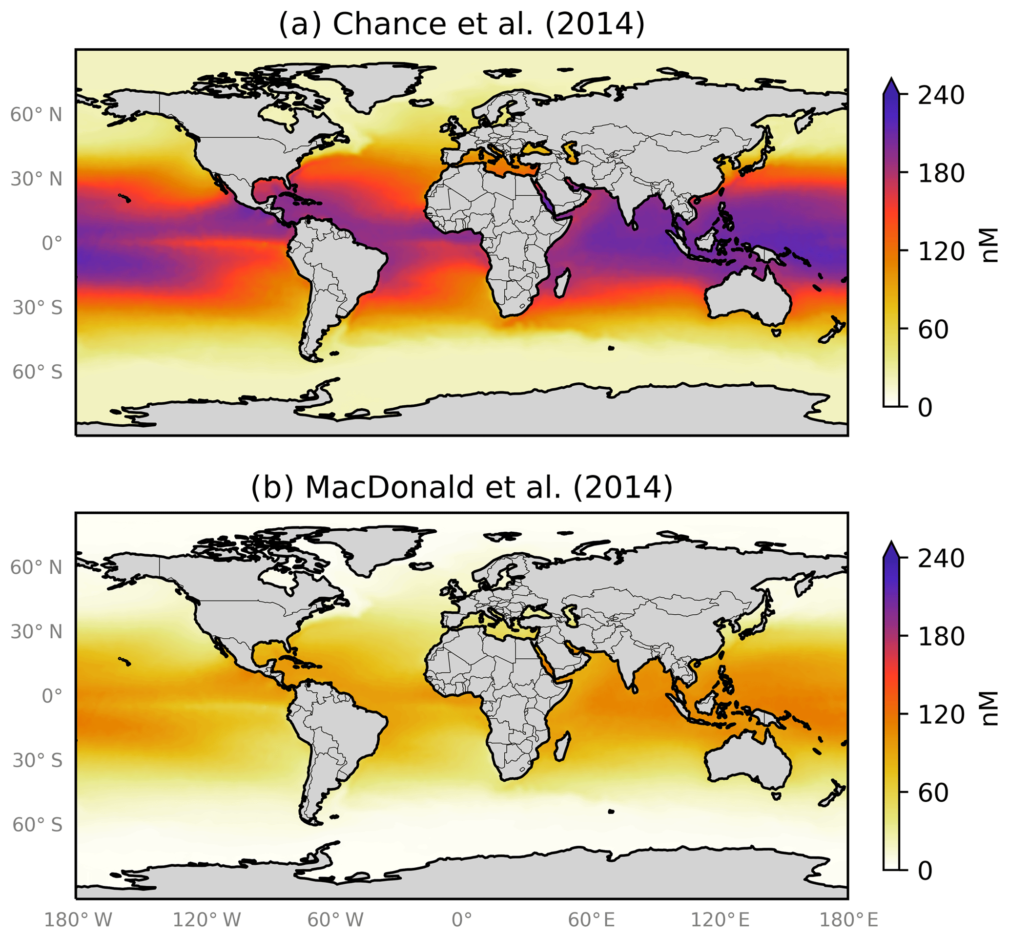
Figure 1Annual average sea-surface iodide concentrations predicted by (a) Eq. (1) from Chance et al. (2014) and (b) Eq. (2) from MacDonald et al. (2014). Temperature fields used to make spatial predictions were from the World Ocean Atlas (Locarnini et al., 2013). Earth raster and vector map data used are freely available from Natural Earth (http://www.naturalearthdata.com/, last access: 23 July 2019).
图1由(a)式预测的年平均海面碘化物浓度( 1 ) 来自Chance 等人。 ( 2014 )和(b)等式。 ( 2 )来自麦克唐纳等人。 ( 2014 ) 。用于进行空间预测的温度场来自世界海洋地图集( Locarnini 等, 2013 ) 。使用的地球栅格和矢量地图数据可从 Natural Earth 免费获取( http://www.naturalearthdata.com/ ,最后访问日期:2019 年 7 月 23 日)。
洛卡尔尼尼等人。 (2013)Zweng 等人。 (2013)加西亚等人。 (2010)贝克尔等人。 (2009)Smith 和 Sandwell (1997)Garcia 等人。 (2014)加西亚等人。 (2014)加西亚等人。 (2014)OBPG (2014)Monterey 和 Levitus (1997)Large 和 Yeager (2009)
Table 1Ancillary variables extracted onto a global
表1提取到全局的辅助变量
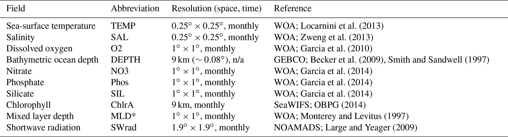
Expansion of Acronyms. WOA: World Ocean Atlas, SeaWIFS: Sea-Viewing Wide Field-of-View Sensor, GEBCO: General Bathymetric Chart of the Oceans, NOAMADS: NOAA National Operational Model Archive and Distribution System. (*) Three available mixed layer depth (MLD) definitions in WOA (vd: variable potential density, pt: potential temperature, pd: potential density) were processed from comma-separated value (CSV) to NetCDF files and extracted. Following Chance et al. (2014), the monthly sum and maximum MLD was also computed (vd, pt, pd) and used for building predictions of iodide. When just the variable MLD is shown, it is MLD as defined by potential temperature. n/a – not applicable
缩写词的扩展。 WOA:世界海洋地图集、SeaWIFS:海景宽视场传感器、GEBCO:海洋通用测深图、NOAMADS:NOAA 国家运行模型档案和分发系统。 (*) WOA 中的三个可用混合层深度 (MLD) 定义(vd:可变电势密度、pt:电势温度、pd:电势密度)从逗号分隔值 (CSV) 处理为 NetCDF 文件并提取。跟随机会等人。 (2014),还计算了每月总和和最大 MLD(vd、pt、pd)并用于构建碘化物的预测。当仅显示变量 MLD 时,它是由位温定义的 MLD。 n/a – 不适用
Considering the need for spatially resolved sea-surface iodide fields by models and the paucity of observations, parameterisations are required that can yield predictions from ancillary variables. This is a regression problem and a number of approaches are available. Conventional linear and linear multi-variant approaches have been used in the past (e.g. see summary in Appendix Table A1). However, they need to assume a functional relationship between the dependent and independent variables. Another approach is machine learning, which uses algorithms to build predictive models. These algorithms take a different approach and use a non-parametric formulation. Machine learning approaches range from interpretable options such as the random forest algorithm (Breiman, 2001) to less interpretable ones such as artificial neural networks (Gardner and Dorling, 1998). On the more interpretable end, machine learning algorithms are being used increasingly within environmental sciences, with recent examples including linear ridge regression and random forest models to replace computationally expensive processes (Keller and Evans, 2019; Nowack et al., 2018) and Gaussian process emulation to explore model biases on a global scale (Lee et al., 2011; Revell et al., 2018).
考虑到通过模型对海面碘化物场进行空间解析的需要以及观测的缺乏,需要进行参数化以从辅助变量中产生预测。这是一个回归问题,有多种方法可用。过去已经使用了传统的线性和线性多变量方法(例如参见附录表A1中的总结)。然而,他们需要假设因变量和自变量之间存在函数关系。另一种方法是机器学习,它使用算法来构建预测模型。这些算法采用不同的方法并使用非参数公式。机器学习方法的范围从可解释的选项(例如随机森林算法( Breiman , 2001 ))到难以解释的选项(例如人工神经网络( Gardner 和 Dorling , 1998 )) 。从更容易解释的角度来看,机器学习算法在环境科学中的使用越来越多,最近的例子包括线性岭回归和随机森林模型,以取代计算成本高昂的过程( Keller 和 Evans , 2019 ; Nowack 等人, 2018 )和高斯过程通过仿真探索全球范围内的模型偏差( Lee et al. , 2011 ; Revell et al. , 2018 ) 。
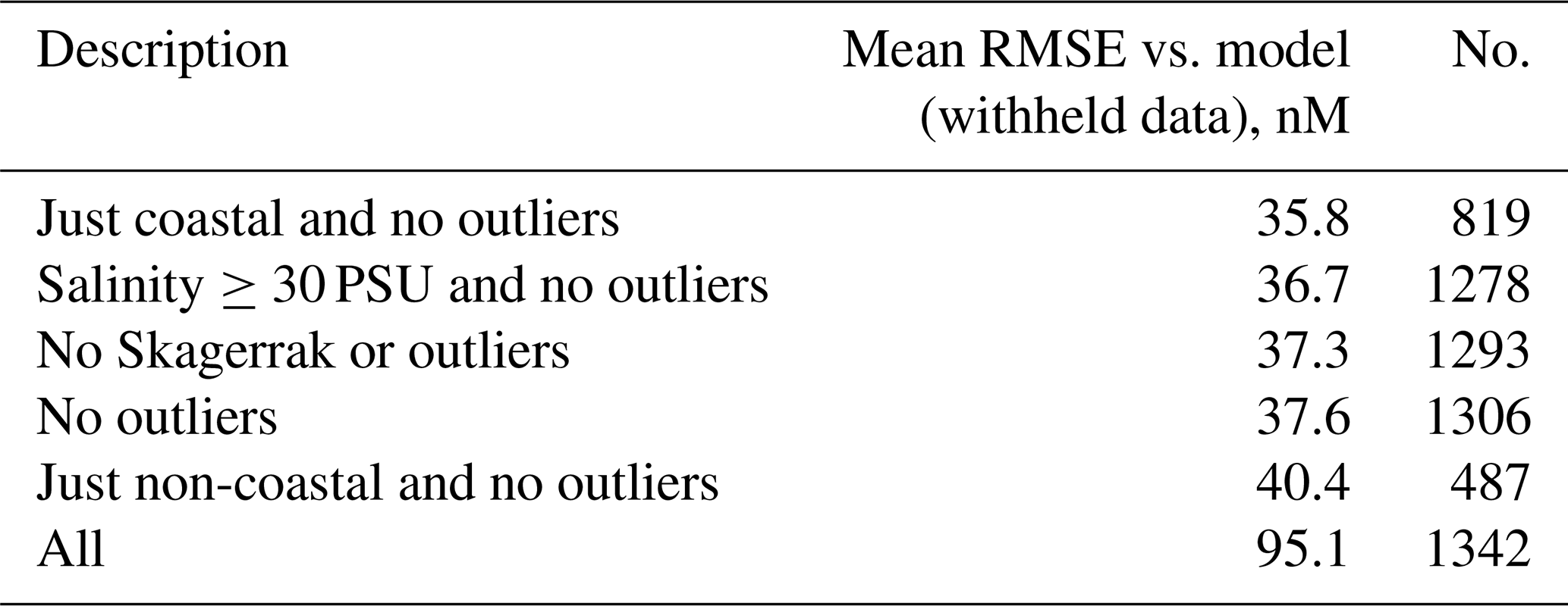
Table 2Splits of dataset used to evaluate outliers and their performance against the withheld data. The root mean square error (RMSE) statistic given as the mean of the performance against the withheld data for 20 different models built from 20 different pseudo-random initialisations (Sect. 3.2). The model used here includes ancillary variables of temperature, depth, and salinity which were thought to intuitively give a reasonable result. “No.” gives the number of samples in each dataset.
表 2用于评估异常值及其针对保留数据的性能的数据集分割。均方根误差 (RMSE) 统计量作为根据 20 个不同伪随机初始化构建的 20 个不同模型的保留数据的性能平均值给出(第3.2节)。这里使用的模型包括温度、深度和盐度等辅助变量,这些变量被认为可以直观地给出合理的结果。 “不。”给出每个数据集中的样本数。
Here, we use a recently expanded compilation of sea-surface iodide observations (Chance et al., 2019a) to build a new sea-surface iodide parameterisation using a data-driven machine learning approach. We choose to use the random forest regressor (RFR) algorithm (Breiman, 2001; Pedregosa et al., 2011), which is relatively simple and produces results that are also easy to understand. We aim to be able to predict global sea-surface iodide based on observations and ancillary physical and chemical variables (e.g. sea-surface temperature, depth, and salinity) from a number of publicly available sources. We first describe the input datasets we use (Sect. 2), then we explain the methodology taken (Sect. 3), and finally we present the predictions at observational locations and globally (Sect. 4). This product should be considered a present-day climatology representing the period of the iodide observations (1967–2018), which we envisage could be useful in applications such as climate and air-quality modelling. We make the resulting high-resolution, global, monthly dataset of predicted iodide available to the community (Sherwen et al., 2019; https://doi.org/10/gfv5v3). When new observations become available, they will be incorporated into the model, and updated versions will be provided through a “living data” model.
在这里,我们使用最近扩展的海面碘化物观测数据汇编( Chance 等人, 2019 a ),利用数据驱动的机器学习方法构建新的海面碘化物参数化。我们选择使用随机森林回归(RFR)算法( Breiman , 2001 ; Pedregosa 等人, 2011 ) ,该算法相对简单,产生的结果也很容易理解。我们的目标是能够根据来自许多公开来源的观测结果和辅助物理和化学变量(例如海面温度、深度和盐度)来预测全球海面碘化物。我们首先描述我们使用的输入数据集(第2节),然后解释所采用的方法(第3节),最后我们提出观测位置和全球的预测(第4节)。该产品应被视为代表碘化物观测时期(1967-2018)的当今气候学,我们认为它可用于气候和空气质量建模等应用。我们向社区提供由此产生的高分辨率、全球、每月预测碘化物数据集( Sherwen 等人, 2019 ; https://doi.org/10/gfv5v3 )。当新的观测结果可用时,它们将被纳入模型中,并通过“实时数据”模型提供更新版本。
2输入数据集
Chance et al. (2019a) provides a compilation of the available 1342 sea-surface (<20 m depth) iodide observations between 1967 and 2018. The dataset is available from the British Oceanographic Data Centre (BODC, Chance et al., 2019b; https://doi.org/10/czhx). It includes 45 % more data points, and has greater spatial coverage, than the previous compilation of 925 observations (Chance et al., 2014). Observations are categorised in Chance et al. (2019a) as “coastal” or “non-coastal”, according to the designation of their static Longhurst biogeochemical province (Longhurst, 1998). We adopt the same categorisation here. This sea-surface iodide dataset then forms the dependent variable for our regression. We assume no inter-annual variability and use all data from all years (1967–2018) in this work.
机会等人。 ( 2019 a )提供了 1967 年至 2018 年间可用的 1342 个海面( <20 m 深度)碘化物观测数据的汇编。该数据集可从英国海洋数据中心获取(BODC、 Chance 等人, 2019 b ; https: //doi.org/10/czhx )。与之前的 925 个观测数据相比,它包含的数据点多了 45%,空间覆盖范围也更大( Chance 等人, 2014 年) 。 Chance 等人对观察结果进行了分类。 ( 2019a )根据其静态朗赫斯特生物地球化学省的指定,分为“沿海”或“非沿海” ( Longhurst , 1998 ) 。我们在这里采用相同的分类。然后,该海面碘化物数据集形成了我们回归的因变量。我们假设没有年际变化,并在这项工作中使用所有年份(1967-2018)的所有数据。
We require a number of physical, chemical, and biological parameters as the independent variables in our regression models. Consistent in situ measurement of these parameters are not available for the iodide observations. Thus we have used a number of ancillary datasets (Table 1) to provide this information. There are a number of criteria for these datasets: they need to be available at an appropriately similar resolution as a gridded product to the desired resolution of the predicted fields, they need to represent potential processes that could control iodide concentrations, and they need to be in some way orthogonal to the other independent variables. Gridded datasets of dissolved organic carbon (e.g. Roshan and DeVries, 2017) and phytoplankton primary productivity (e.g. Behrenfeld and Falkowski, 1997) may have some usefulness, but they themselves are built using statistical models with other variables and thus we do not use those here. The selected ancillary variables (Table 1) were first extracted from their native resolution using the nearest-neighbour method onto a consistent high-resolution monthly grid (
我们需要许多物理、化学和生物参数作为回归模型中的自变量。这些参数的一致原位测量不适用于碘化物观测。因此,我们使用了许多辅助数据集(表1 )来提供此信息。这些数据集有许多标准:它们需要以与预测场所需分辨率适当相似的网格产品的分辨率提供,它们需要代表可以控制碘化物浓度的潜在过程,并且它们需要以某种方式与其他自变量正交。溶解有机碳(例如Roshan 和 DeVries , 2017 )和浮游植物初级生产力(例如Behrenfeld 和 Falkowski , 1997 )的网格数据集可能有一些用处,但它们本身是使用具有其他变量的统计模型构建的,因此我们在这里不使用它们。首先使用最近邻法将选定的辅助变量(表1 )从其原始分辨率中提取到一致的高分辨率每月网格上(
For each iodide observation, the nearest point in space and time was extracted from the high-resolution gridded ancillary data. For the 31 iodide observations where a month was not available (Luther and Cole, 1988; Tsunogai and Henmi, 1971; Wong and Cheng, 1998), an arbitrary month was chosen (of March for northern hemispheric observations and September for southern hemispheric observations). Outliers within the observations are removed as described in Sect. 3.3. A further single dataset (Truesdale et al., 2003) was also excluded from this analysis. This is discussed in Appendix Sect. A1.
对于每个碘化物观测,从高分辨率网格辅助数据中提取空间和时间上最近的点。对于无法获得月份的 31 个碘化物观测( Luther 和 Cole , 1988 ; Tsnogai 和 Henmi , 1971 ; Wong 和 Cheng , 1998 ) ,选择任意月份(北半球观测为 3 月,南半球观测为 9 月) 。观察中的异常值被删除,如第 1 节中所述。 3.3 .另一个单一数据集( Truesdale 等人, 2003 )也被排除在该分析之外。这在附录部分讨论。 A1 。
3方法
Here we first explain the way in which we use the machine learning algorithm (Sect. 3.1). We then explain how we have calculated uncertainty (Sect. 3.2), how observations considered outliers have been removed from the data (Sect. 3.3), and how we have decided which ancillary variables (temperature, salinity, etc.) to use as independent variables for an ensemble prediction (Sect. 3.4). Finally we describe the interpretable ensemble prediction model that results from this methodology in both numerical and graphical terms (Sect. 3.5).
这里我们首先解释一下我们使用机器学习算法的方式(第3.1节)。然后,我们解释如何计算不确定性(第3.2节),如何从数据中删除被视为异常值的观测值(第3.3节),以及我们如何决定使用哪些辅助变量(温度、盐度等)作为独立变量集合预测的变量(第3.4节)。最后,我们用数值和图形术语描述了由这种方法产生的可解释的集合预测模型(第3.5节)。
3.1 Random forest regressor algorithm
3.1随机森林回归器算法
As the aim here is to predict a continuous numerical value for sea-surface iodide, a regression approach is taken. As discussed in the introduction, previous approaches have been made to parameterise sea-surface iodide, and the most commonly used relationships employ sea-surface temperature as the predictor variable. Here we take a different multivariate and non-parametric approach, using the computationally cheap and interpretable random forest regressor (RFR) algorithm (Breiman, 2001; Pedregosa et al., 2011).
由于此处的目的是预测海面碘化物的连续数值,因此采用回归方法。正如引言中所讨论的,之前已经采用了参数化海面碘化物的方法,最常用的关系式采用海面温度作为预测变量。在这里,我们采用不同的多变量和非参数方法,使用计算成本低且可解释的随机森林回归(RFR)算法( Breiman , 2001 ; Pedregosa 等人, 2011 ) 。
Random forest regression is based on finding a number of decisions trees, which predict the dependent variable. All of the trees contribute to the prediction, and they are collectively referred to as a “forest”. These trees can be explained as a record of the way the algorithm has linearly traversed a subset of the training data, splitting the data into two parts at each decision point or “node” in a way that minimised the internal differences of the parts. The best split is chosen between the available variables based on an error metric (e.g. mean square error), and this process is continued until a criterion of purity is reached or a minimum number of data points are left from a split. This is essentially a classification problem. The prediction of the forest is the mean value of the prediction of all of the different decision trees, which attempts to make the results more of a regression problem. More details of this approach can be found in Friedman et al. (2009).
随机森林回归基于查找多个决策树,这些决策树预测因变量。所有树木都对预测做出贡献,它们统称为“森林”。这些树可以解释为算法线性遍历训练数据子集的方式的记录,在每个决策点或“节点”将数据分成两部分,以最小化各部分内部差异的方式。基于误差度量(例如均方误差)在可用变量之间选择最佳分割,并且继续该过程直到达到纯度标准或分割留下最小数量的数据点。这本质上是一个分类问题。森林的预测是所有不同决策树的预测的平均值,它试图使结果更像是一个回归问题。有关此方法的更多详细信息,请参见Friedman 等人。 ( 2009 ) 。
This approach differs from previous approaches which have individually tested proposed relationships and selected the best-performing model(s) as a parameterisation (e.g. Table A1). Here, an algorithm uses the data it is provided to build a model that gives a prediction, and therefore it is the data themselves that define the model that is used to predict new values. A key difference of this approach is also that only a subset, the training set, is used to build the model, and the rest (or withheld set) is then used to test the performance of the model. Here we use 80 % of the data for the training set and use the remaining 20 % as the withheld set (also commonly referred to as the “testing set”).
该方法不同于先前的方法,先前的方法单独测试了所提出的关系并选择性能最佳的模型作为参数化(例如表A1 )。在这里,算法使用所提供的数据来构建给出预测的模型,因此数据本身定义了用于预测新值的模型。这种方法的一个关键区别还在于,仅使用一个子集(训练集)来构建模型,然后使用其余部分(或保留集)来测试模型的性能。这里我们使用 80% 的数据作为训练集,使用剩余的 20% 作为保留集(通常也称为“测试集”)。
To ensure that the models built are generalisable and mitigate overfitting, the random forest approach used here artificially increases the randomness within the forest (Pedregosa et al., 2011). This is done by randomly combining single decision trees by an approach referred to as “bootstrap aggregation” or “bagging” (Breiman, 2001; Tong et al., 2003). This additional bagging approach randomly samples observations within the training dataset and so mitigates overfitting of the trees to the dataset (Friedman et al., 2009). Furthermore, a stratified sampling approach was taken. Specifically, the overall dataset was split into quartiles according to iodide concentration value, and training data were randomly selected from each quartile. This approach was used to maintain the same statistical distribution in the training/testing data as the overall dataset.
为了确保建立的模型具有普适性并减轻过度拟合,这里使用的随机森林方法人为地增加了森林内的随机性( Pedregosa et al. , 2011 ) 。这是通过称为“引导聚合”或“装袋”的方法随机组合单个决策树来完成的( Breiman , 2001 ; Tong 等人, 2003 ) 。这种额外的装袋方法对训练数据集中的观察结果进行随机采样,从而减轻了树与数据集的过度拟合( Friedman 等人, 2009 ) 。此外,还采取了分层抽样的方法。具体来说,根据碘化物浓度值将整个数据集分成四分位数,并从每个四分位数中随机选择训练数据。这种方法用于保持训练/测试数据与整个数据集相同的统计分布。
Machine learning algorithms can generally be tuned to increase performance using settings called hyperparameters. However, random forests are known to generally perform well without tuning. The default hyperparameters were therefore used here (Pedregosa et al., 2011), except for increasing the number of trees (“n_estimators”) from 10 to 500. Mean square error (MSE) was used as the criterion for evaluating each split (also referred to as a “node”). The maximum number of “features” (the ancillary variables provided to the algorithm, such as temperature or nitrate concentration) considered when looking for the best split is set to the number provided to the algorithm. The number of splits a tree is allowed to make (“max_depth”) is not restricted, and further nodes are made until leaves contain less than two samples (“min_samples_split”) and a minimum of one (“min_samples_leaf”). All the random forest models are built using bootstrapping.
通常可以使用称为超参数的设置来调整机器学习算法以提高性能。然而,众所周知,随机森林通常无需调整即可表现良好。因此,这里使用默认的超参数( Pedregosa et al. , 2011 ) ,除了将树的数量(“n_estimators”)从 10 增加到 500 之外。均方误差(MSE)被用作评估每个分割的标准(也称为“节点”)。寻找最佳分割时考虑的“特征”(提供给算法的辅助变量,例如温度或硝酸盐浓度)的最大数量设置为提供给算法的数量。允许树进行分割的数量(“max_depth”)不受限制,并且会生成更多节点,直到叶子包含少于两个样本(“min_samples_split”)且至少包含一个样本(“min_samples_leaf”)。所有随机森林模型都是使用引导构建的。
3.2 Error and uncertainty calculations
3.2误差和不确定性计算
Understanding the errors and uncertainties in the global iodide distribution is important due to any sensitivities to this value within the modelled Earth system. We consider three sources of error in our predictions: the “dataset selection” error due to the splitting of the dataset into training and withheld parts, the “model selection error” due to the choice of dependent variables, and the “observational error” on the iodide measurements.
由于模拟地球系统内对该值的敏感性,了解全球碘化物分布的误差和不确定性非常重要。我们在预测中考虑三个误差来源:由于将数据集分为训练部分和保留部分而导致的“数据集选择”误差,由于因变量的选择而导致的“模型选择误差”,以及由于变量的选择而导致的“观察误差”碘化物测量。
To quantify the range of the dataset selection error, we construct models from 20 pseudo-random splits of the dataset into training and withheld parts. The hyperparameters and input ancillary variables are kept the same for the generation of the 20 models, so that the only difference between the models is the training dataset. These 20 models are then used to predict the withheld data. Performance metrics (e.g. root mean square error (RMSE) and average absolute prediction) can then be calculated for each model. This gives a range of 20 values, which can then be converted to a percentage range as the error. This is done by dividing the largest range in predicted values for a model by the minimum predicted value, to give a maximum value for the range of error, and then taking the smallest range in the predicted values and dividing this by the maximum value, to give a minimum value for the error range. Significant differences between the model's performance metrics would suggest important sensitivity to the training/withheld dataset splits.
为了量化数据集选择误差的范围,我们将数据集的 20 个伪随机分割构建为训练部分和保留部分。生成 20 个模型时,超参数和输入辅助变量保持相同,因此模型之间的唯一区别是训练数据集。然后使用这 20 个模型来预测保留的数据。然后可以计算每个模型的性能指标(例如均方根误差(RMSE)和平均绝对预测)。这给出了 20 个值的范围,然后可以将其转换为百分比范围作为误差。这是通过将模型预测值的最大范围除以最小预测值来完成的,以给出误差范围的最大值,然后取预测值的最小范围并将其除以最大值,得到给出误差范围的最小值。模型性能指标之间的显着差异表明对训练/保留数据集分割的重要敏感性。
We define the “model selection” error as the uncertainty resulting from the choice of input ancillary variables. A number of combinations of input variables are possible in generating the models, and each will generate a different prediction. We quantify this error as the difference in performance against the withheld dataset and prediction value (e.g. average global value). Similarly to our calculation of the dataset selection error, this can be converted to percentage error by considering the range in these values and dividing them by minimum and maximum values.
我们将“模型选择”误差定义为由于选择输入辅助变量而产生的不确定性。在生成模型时可以使用多种输入变量组合,并且每种组合都会生成不同的预测。我们将此误差量化为与保留数据集和预测值(例如平均全局值)的性能差异。与我们计算数据集选择误差类似,可以通过考虑这些值的范围并将它们除以最小值和最大值来将其转换为百分比误差。
For the observational error we refer to Chance et al. (2019a), who provide individual error estimates for each of the iodide observations in the data compilation. Over half (51 %) of the data points have an error of 5 % or less, and a further ∼25 % have an uncertainty in the range of 5 %–10 %. We therefore use a value of 10 % as a conservative estimate of the observational error.
对于观察误差,我们参考Chance 等人。 ( 2019 a ) ,他们为数据汇编中的每个碘化物观测值提供了单独的误差估计。超过一半 (51%) 的数据点的误差为 5% 或更少,另外约 25 % 的数据点的不确定性在 5%–10% 范围内。因此,我们使用 10% 的值作为观测误差的保守估计。
3.3 Outlier identification and removal
3.3异常值识别和去除
Our dataset consists of values for ancillary variables and iodide concentration for all of the 1342 measurement locations in the observational dataset (Sect. 2). As discussed in Sect. 3.1, we split this dataset into two parts: (i) a training set for use in building and optimising models, and (ii) a withheld set to evaluate the models built. Particular care was taken to ensure the withheld and training datasets were representative of the entire dataset in the way the models are built, therefore improving performance and generalisability to unseen data (see Sect. 3.1).
我们的数据集由观测数据集中所有 1342 个测量位置的辅助变量值和碘化物浓度组成(第2节)。正如第 3 节中所讨论的那样。 3.1中,我们将该数据集分为两部分:(i)用于构建和优化模型的训练集,以及(ii)用于评估构建的模型的保留集。我们特别注意确保保留数据集和训练数据集以模型构建的方式代表整个数据集,从而提高性能和对未见数据的通用性(参见第3.1节)。
We take a random forest regressor model built with variables that were intuitively assumed to give a reasonable ability to differentiate the observations (using depth, temperature, and salinity as the independent variables – abbreviated to “RFR(DEPTH+TEMP+SAL)” following Table 1). The RFR(DEPTH+TEMP+SAL) model was then used to explore the variation of error in the predictions using the dataset selection error approach described in Sect. 3.2. This builds multiple versions of the same model with different splits of training and test data and yields a distribution of root mean square error in the predicted iodide for withheld data as summarised in the final column of Table 2 and shown graphically in Appendix Fig. A1.
我们采用随机森林回归模型,该模型使用变量构建,直观地假设这些变量具有区分观测结果的合理能力(使用深度、温度和盐度作为自变量 - 缩写为“RFR(DEPTH+TEMP+SAL)”,如下表1 )。然后使用 RFR(DEPTH+TEMP+SAL) 模型来探索预测中误差的变化,使用第 1 节中描述的数据集选择误差方法。 3.2 .这使用不同的训练和测试数据分割构建了同一模型的多个版本,并产生了保留数据的预测碘化物的均方根误差分布,如表2最后一列中总结并在附录图A1中以图形方式显示。
We define outliers here as values greater than the third quartile plus 1.5 times the interquartile range (Frigge et al., 1989). Removing these 49 values categorised as outliers (>309.5 nM) leads to a vast improvement in the RMSE error in the ensemble prediction from 95.1 to 37.6 nM (Table 2). This is shown graphically in Appendix Fig. A1, with the other subsets of the data explored (Table 2). This demonstrates that the high values are not well enough represented by the dataset to be able to be captured by the RFR approach. The removal of these high values from the dataset can also be justified as the driver for these concentrations is not yet well understood (Chance et al., 2014, 2019c; Cutter et al., 2018).
我们在这里将异常值定义为大于第三个四分位数加上 1.5 倍四分位距的值( Frigge 等, 1989 ) 。删除这 49 个被分类为异常值 ( >309.5 nM) 的结果是,集合预测中的 RMSE 误差从 95.1 nM 大幅改善至 37.6 nM(表2 )。附录图A1中以图形方式显示了这一点,并探索了其他数据子集(表2 )。这表明数据集不足以很好地表示高值,无法通过 RFR 方法捕获。从数据集中删除这些高值也是合理的,因为这些浓度的驱动因素尚未得到很好的理解( Chance 等人, 2014,2019 c ; Cutter 等人, 2018 ) 。
Removing these outliers reduces RMSE in the prediction with the 20 independent model builds from 48.2 to 2.3 nM (third quartile–first quartile). Once these outliers are excluded, more modest changes in average RMSE are then seen if models are built only using coastal or non-coastal data. Figure A1 also shows this is seen when removing lower salinity data (“Salinity ≥30 PSU and no outliers”), which is indicative of estuarine water. This highlights the strength in this approach's ability to predict iodide in different biogeochemical regions (i.e. not just coastal or non-coastal locations).
删除这些异常值可将 20 个独立模型构建的预测中的 RMSE 从 48.2 降低到 2.3 nM(第三个四分位数 - 第一个四分位数)。一旦排除这些异常值,如果仅使用沿海或非沿海数据构建模型,则平均 RMSE 会出现更温和的变化。图A1还显示了在删除较低盐度数据(“盐度≥30 PSU 并且没有异常值”)时看到的情况,这表明是河口水。这凸显了该方法预测不同生物地球化学区域(即不仅仅是沿海或非沿海地区)碘化物的能力。
An additional removal of a single dataset of 19 observations from the Skagerrak strait (Truesdale et al., 2003) was made due to it exerting a disproportionate influence on iodide prediction in high northern latitudes (
额外删除了斯卡格拉克海峡的 19 个观测值的单个数据集( Truesdale 等, 2003 ),因为它对北高纬度地区的碘化物预测产生了不成比例的影响(
From here, only the 1293 observational points excluding outliers and the data from the Skagerrak strait (Truesdale et al., 2003) are used.
从这里开始,仅使用排除异常值的 1293 个观测点和斯卡格拉克海峡的数据( Truesdale 等, 2003 ) 。
3.4 Selection of ancillary variables and building an ensemble prediction
3.4辅助变量的选择和建立集合预测
To decide which ancillary variables (temperature, salinity, etc.; see Table 1 and Sect. 2) should be used to predict sea-surface iodide concentration, RFR models were built and evaluated with different combinations of variables. Thirty eight combinations were considered (see first column of Appendix Table A2).
为了确定应使用哪些辅助变量(温度、盐度等;参见表1和第2节)来预测海面碘化物浓度,建立了 RFR 模型并使用不同的变量组合进行评估。考虑了 38 种组合(参见附录表A2第一列)。
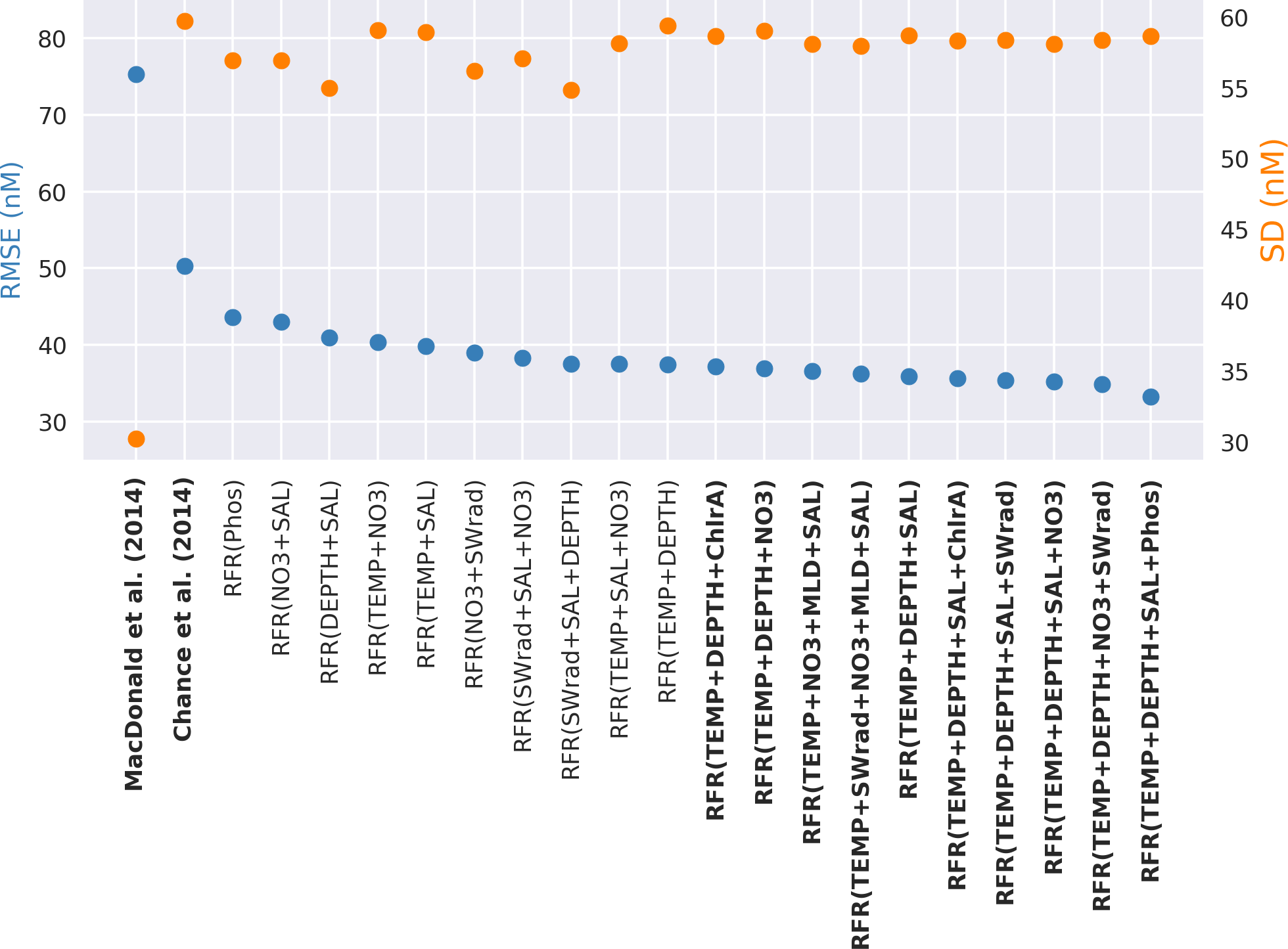
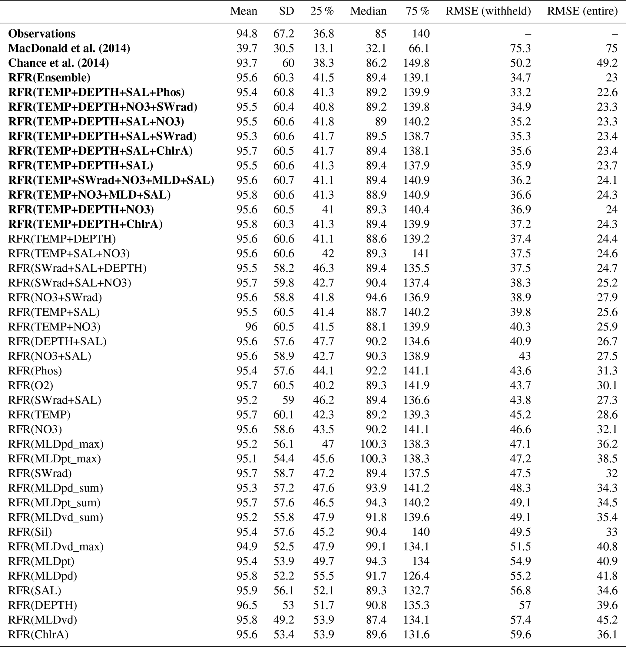
The top 20 performing models, based on their root mean square error against the withheld data, are plotted in Fig. 2, alongside existing parameterisations. The standard deviation for all predicted values is also shown to illustrate variation in the predictions. A complete list of the performance and of all models built here and their performance is given in the appendix (Table A2).
根据保留数据的均方根误差,表现最好的 20 个模型与现有参数一起绘制在图2中。还显示所有预测值的标准差以说明预测的变化。附录(表A2 )中给出了此处构建的所有模型及其性能的完整列表。
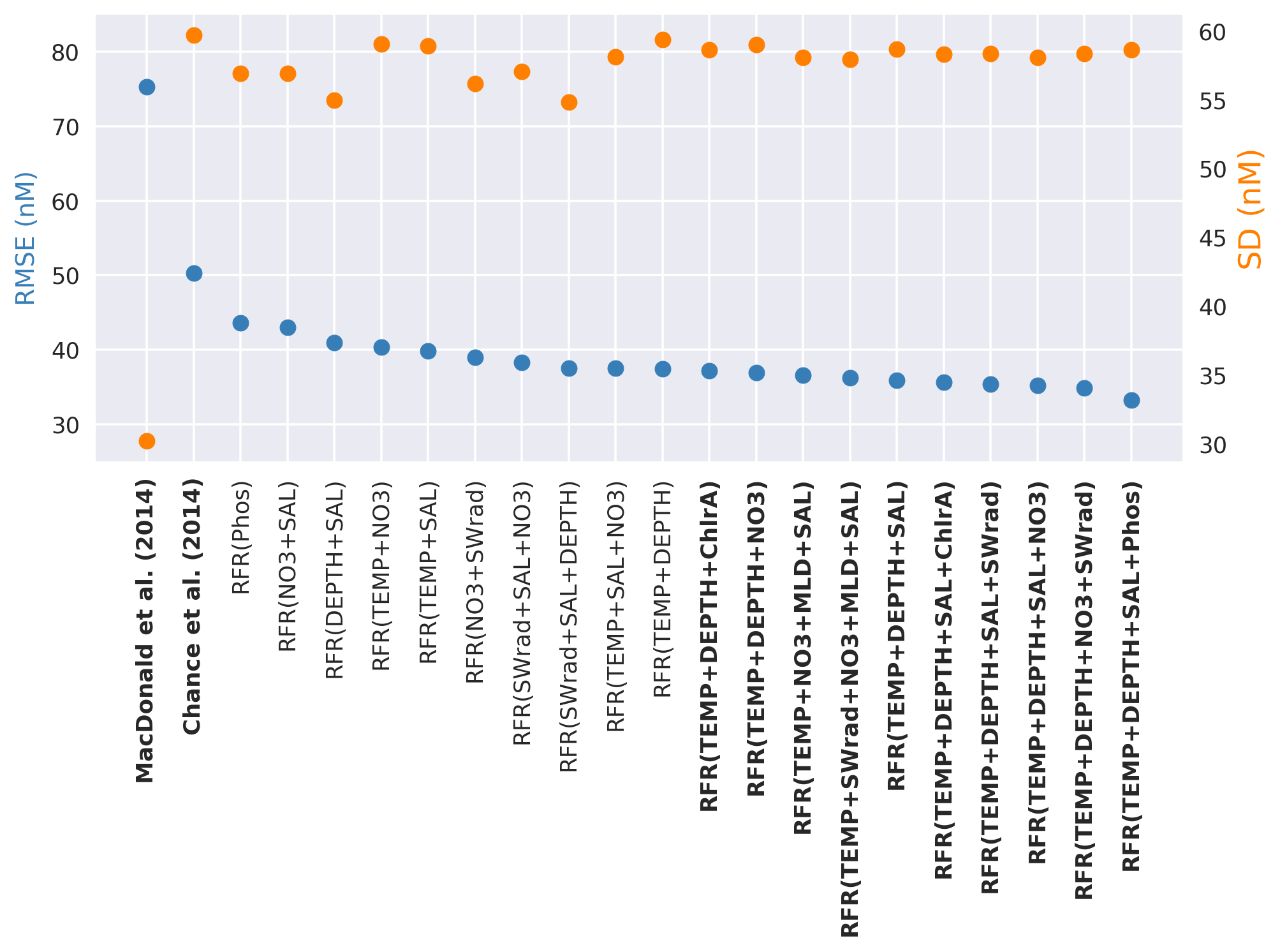
Figure 2Random forest regression (RFR) model performance (root mean square error (RMSE), blue) against the withheld data for the top 20 models on the left-hand y axis, along with values from the parameterisations from Chance et al. (2014) and MacDonald et al. (2014). The right-hand y axis is standard deviation of the prediction for the withheld data (orange). The top 10 performing models and the two exiting parameterisations considered here (Chance et al., 2014; MacDonald et al., 2014) are shown in bold. Parameterisations are ordered by their RMSE. Abbreviations are given in Table 1.
图 2随机森林回归 (RFR) 模型性能(均方根误差 (RMSE),蓝色)与左侧y轴上前 20 个模型的保留数据,以及来自Chance 等人的参数化的值。 ( 2014 )和麦克唐纳等人。 ( 2014 ) 。右侧y轴是保留数据(橙色)的预测的标准偏差。这里考虑的前 10 个性能模型和两个现有参数化( Chance 等人, 2014 年; MacDonald 等人, 2014 年)以粗体显示。参数化按其 RMSE 排序。表1中给出了缩写。
The RMSE values in Fig. 2 show the increased skill present in the new predictions compared to the existing parameterisations. The RMSE improves from the 75.3 and 50.2 nM found for the Chance et al. (2014) and MacDonald et al. (2014) parameterisations, respectively, to 33.2–37.4 nM for the top 10 models created here. Only modest gains are seen in RMSE between models with three variables or more.
图2中的 RMSE 值显示,与现有参数化相比,新预测中的技巧有所提高。 RMSE 较Chance 等人发现的 75.3 和 50.2 nM 有所提高。 ( 2014 )和麦克唐纳等人。 ( 2014 )将此处创建的前 10 个模型的参数分别设置为 33.2–37.4 nM。具有三个或更多变量的模型之间的 RMSE 仅出现适度的增长。
The best-performing model in the list is only marginally better than the 10th best-performing one; therefore there is not an obvious “best” performing set of ancillary variables. Thus going forward we use an ensemble prediction approach based on the mean value from an ensemble of the 10 top-performing models.
列表中性能最好的模型仅比性能排名第 10 的模型稍好一些;因此,不存在明显的“最佳”表现辅助变量集。因此,接下来我们将使用基于 10 个表现最好的模型的集合平均值的集合预测方法。
3.5 Model descriptions
3.5型号说明
Unlike many machine learning approaches, the random forest regressor algorithm is interpretable. The decision trees can be visualised to explain the main features driving the splits. Figure 3 shows schematically the whole regression approach taken here. Panel (a) shows single trees, of which 500 are built with the same input variables and then combined into forest (b). Then this forest is combined with the nine other top-performing models (made from different combinations of ancillary variables) to make an ensemble (c). The 10 predictions of (c) are then arithmetically averaged into a single prediction, which thus includes the predictions of 5000 trees with 10 different combinations of input variables. In Fig. 3a, the colour of a limb or “branch” following a node is given by the variable driving that split within the training dataset. For Fig. 3b and c it shows the percent of times that a variable drives that node within the forest. The value of the ancillary variable that sets the split is shown inside the circle (a, b, c). The thickness of the branch scales to the throughput of training dataset samples contained within that split. The trees are shown to a depth of five nodes for aesthetic reasons and due to increased divergence of the trees within a forest the deeper you go. However the trees themselves are unlimited in the depth they can reach.
与许多机器学习方法不同,随机森林回归算法是可解释的。决策树可以可视化来解释驱动分裂的主要特征。图3示意性地显示了此处采用的整个回归方法。面板 (a) 显示单棵树,其中 500 棵使用相同的输入变量构建,然后组合成森林 (b)。然后将该森林与其他九个表现最好的模型(由辅助变量的不同组合组成)组合起来形成一个集合(c)。然后,(c) 的 10 个预测被算术平均为单个预测,从而包括具有 10 种不同输入变量组合的 5000 棵树的预测。在图3a中,节点后面的肢体或“分支”的颜色由训练数据集中分割的变量驱动给出。对于图3 b 和 c,它显示了变量驱动森林中该节点的次数百分比。设置分割的辅助变量的值显示在圆圈内(a、b、c)。分支的厚度与该分割中包含的训练数据集样本的吞吐量成比例。出于美观原因,树木显示为五个节点的深度,而且随着深度的加深,森林内树木的发散性也会增加。然而,树木本身的深度是无限的。

Figure 3Schematic illustration of how (a) multiple decision trees are combined into (b) a forest and then combined into (c) a further 10-member ensemble. (a) shows individual trees in a forest. (b) represent a forest of 500 trees as a single figurative tree. (c) shows the 10 forests of 500 trees combined into a single prediction. The branches in plots (a)–(c) are coloured by the percentage of the decisions at a given node that are driven by a given variable. That value within the circle gives the value of the main ancillary variable driving a split. The thickness of branches gives the throughput of the dataset through a given node for single trees (a) or the average for plots of forests (b, c). The 10 forests shown as thumbnails in panel (c) are also shown in larger form in Appendix Fig. A5. Variable names are coloured as per the following coloured text: temperature (blue, ∘C), depth (orange, metres), chlorophyll a (green, mg m−3), salinity (pink, PSU), nitrate (brown, µg m−3), mixed layer depth (MLD; purple, metres), phosphate (red, µg m−3), and shortwave radiation (grey, W m−2).
图 3示意图显示(a)多个决策树如何组合成(b)森林,然后组合成(c)进一步的 10 成员集成。 (a)显示了森林中的单棵树。 (b)将 500 棵树组成的森林表示为一棵象征性的树。 (c)显示将 10 个森林的 500 棵树组合成一个预测。图中(a) – (c)中的分支根据给定节点上由给定变量驱动的决策的百分比进行着色。圆圈内的值给出了驱动分裂的主要辅助变量的值。树枝的粗细给出了单棵树(a)的给定节点的数据集吞吐量或森林图块的平均值(b, c) 。图(c)中以缩略图显示的 10 个森林也在附录图A5中以放大形式显示。变量名称按照以下彩色文本着色:温度(蓝色, ∘ C)、深度(橙色,米)、叶绿素a (绿色,mg m −3 )、盐度(粉红色,PSU)、硝酸盐(棕色, μg m -3 )、混合层深度(MLD;紫色,米)、磷酸盐(红色, μg m -3 )和短波辐射(灰色,W m -2 )。
The first and larger splits in the data at decision nodes in the models can be simply read, which can provide understanding of the main variables driving the initial and largest splits in the prediction. For all models in the ensemble, the initial split is driven by temperature, with a split occurring at around 21.1 ∘C (with a standard deviation of 1.2 ∘C). The data are then split by two further nodes from this, a left- and right-hand split (e.g. Fig. 3b). If depth or temperature is present as a variable, then they drive the majority of the next splits. If depth is not present as a variable, then either nitrate or mixed layer depth (MLD) is the most common variable to dictate the split in the data at the next node in the tree. Thus a qualitative way of interpreting the initial splits of the dataset would be to say that the model is primarily differentiating between warmer and shallower locations.
可以简单地读取模型中决策节点处的数据中的第一个和较大的分割,这可以提供对驱动预测中的初始和最大分割的主要变量的理解。对于系综中的所有模型,初始分裂由温度驱动,分裂发生在 21.1 ∘ C 左右(标准差为 1.2 ∘ C)。然后,数据被另外两个节点分割,即左手分割和右手分割(例如图3 b)。如果深度或温度作为变量存在,那么它们会驱动接下来的大部分分裂。如果深度不作为变量存在,则硝酸盐或混合层深度 (MLD) 是最常见的变量,用于指示树中下一个节点处的数据分割。因此,解释数据集初始分割的定性方法是说该模型主要区分较温暖和较浅的位置。
4 个结果
Here we evaluate the performance of the ensemble prediction against the observational dataset (Sect. 4.1), and then we explore the predicted global monthly surface concentrations (Sect. 4.2).
在这里,我们根据观测数据集评估集合预测的性能(第4.1节),然后我们探索预测的全球每月表面浓度(第4.2节)。
4.1 Prediction of iodide at observational locations
4.1观测地点碘化物预测
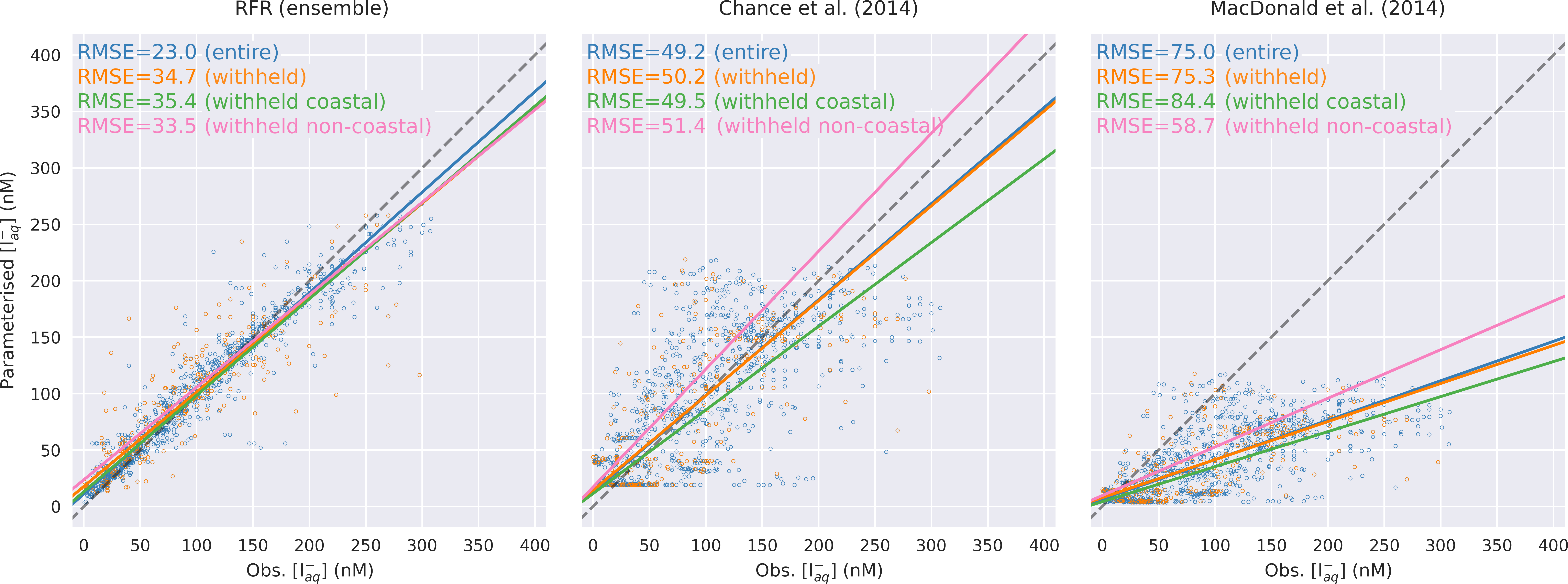
Figure 4 shows a point-by-point comparison between parameterised and observed iodide for the entire dataset, the withheld dataset, and the withheld coastal dataset and withheld non-coastal dataset. Predictions are shown for the ensemble random forest regressor approach described here and for both the Chance et al. (2014) and MacDonald et al. (2014) parameterisations. The root mean square errors of observed and predicted values are given in Fig. 4 and in Table 3.
图4显示了整个数据集、保留数据集、保留沿海数据集和保留非沿海数据集的参数化碘化物和观测到的碘化物之间的逐点比较。显示了此处描述的集成随机森林回归器方法以及Chance 等人的预测。 ( 2014 )和麦克唐纳等人。 ( 2014 )参数化。观测值和预测值的均方根误差如图4和表3所示。

Figure 4Regression plots showing comparisons between predicted values and observations in the entire (blue, N=1293) and withheld data (orange, N=259), withheld data classed as coastal (green, N=157), and the withheld data classed as non-coastal (pink, N=102). Solid lines give the orthogonal distance regression line of best fit. The dashed grey line gives the 1:1 line. Root mean square error for each line is annotated by subplot in nanomolar (nM).
图 4回归图显示了整个数据(蓝色, N = 1293 )和保留数据(橙色, N = 259 )、保留数据归类为沿海(绿色, N = 157 )以及保留数据分类的预测值和观测值之间的比较作为非沿海地区(粉红色, N = 102 )。实线给出最佳拟合的正交距离回归线。灰色虚线表示1:1线。每条线的均方根误差由纳摩尔 (nM) 的子图注释。
机会等人。 (2014) 麦克唐纳等人。 (2014)
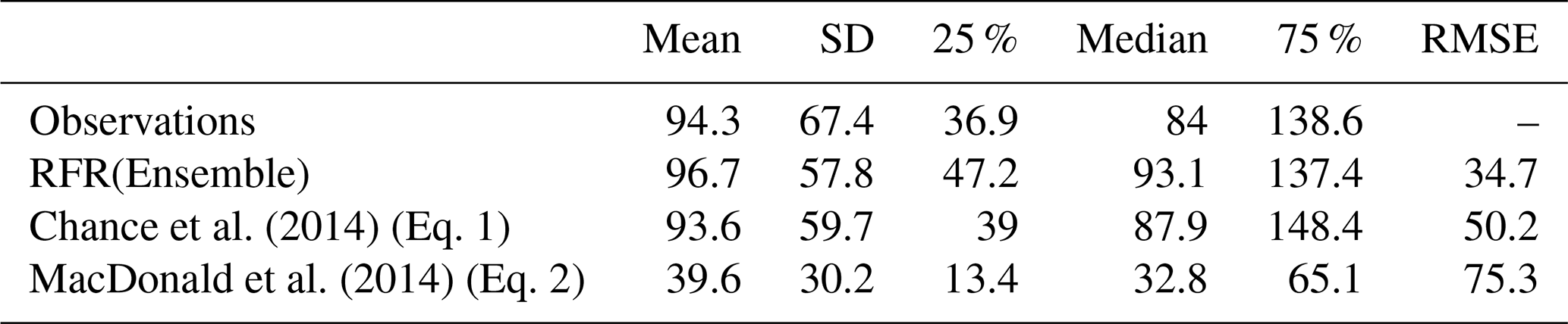
Table 3Statistics for observations and predictions by the ensemble prediction (RFR(ensemble)) and existing parameterisations against the entire dataset of observations. The root mean square error is shown against the entire and the withheld data.
表 3集合预测 (RFR(ensemble)) 的观测值和预测的统计数据以及针对整个观测数据集的现有参数化。显示针对整个数据和保留数据的均方根误差。
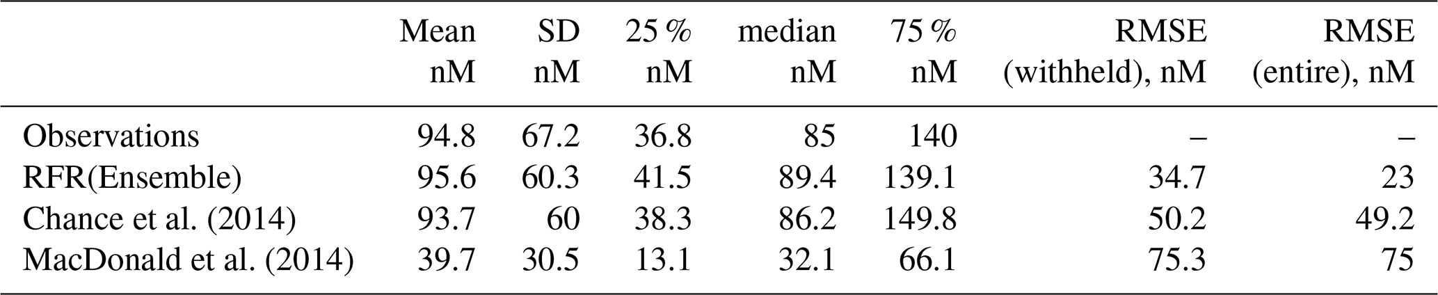
The new ensemble prediction is the best performing, with a lower RMSE (35 nM) compared to the existing parameterisations (75 and 50 nM for the MacDonald et al., 2014, and Chance et al., 2014, respectively) for the withheld data. Both the new parameterisation and Chance et al. (2014) parameterisation are relatively unbiased (both have best-fit-line slopes of 0.84, against the withheld data), but the new parameterisation shows less noise than Chance et al. (2014). MacDonald et al. (2014) shows a significant low bias and significant noise. The improved skill from the RFR ensemble is consistent for both coastal and non-coastal observations.
新的集合预测性能最佳,与保留数据的现有参数化( MacDonald 等人, 2014 年和Chance 等人, 2014 年分别为 75 和 50 nM)相比,RMSE 更低(35 nM) 。新的参数化和Chance 等人。 ( 2014 )参数化相对无偏差(相对于保留的数据,两者的最佳拟合线斜率为 0.84),但新的参数化显示出比Chance 等人更少的噪声。 ( 2014 ) 。麦克唐纳等人。 ( 2014 )显示出显着的低偏差和显着的噪声。 RFR 集合改进的技能对于沿海和非沿海观测都是一致的。
Figure 5 shows comparisons between the probability distribution functions (PDFs) of the observed iodide and the predictions, together with the PDFs of the biases for the entire, coastal, and non-coastal withheld datasets. The PDF of the new parameterisation shows the greatest similarity to the observations. The PDF from Chance et al. (2014) shows a similar range to the observations and structure to the observations, whereas the PDF from MacDonald et al. (2014) shows again a significant underestimate. The bias plots show the new predictions are generally clustered around zero with a relatively narrow peak. Chance et al. (2014) is again roughly clustered around zero but shows a wider peak. The largest biases are found from MacDonald et al. (2014), which systematically underestimates observed iodide concentrations.
图5显示了观测到的碘化物的概率分布函数 (PDF) 与预测之间的比较,以及整个沿海和非沿海保留数据集的偏差 PDF。新参数化的概率密度函数显示出与观测结果的最大相似性。来自Chance 等人的 PDF。 ( 2014 )显示了与观察结果相似的范围和结构,而MacDonald 等人的 PDF。 ( 2014 )再次显示出明显的低估。偏差图显示,新的预测通常聚集在零附近,峰值相对较窄。机会等人。 ( 2014 )再次大致聚集在零附近,但显示出更宽的峰值。最大的偏见来自麦克唐纳等人。 ( 2014 ) ,系统地低估了观测到的碘化物浓度。
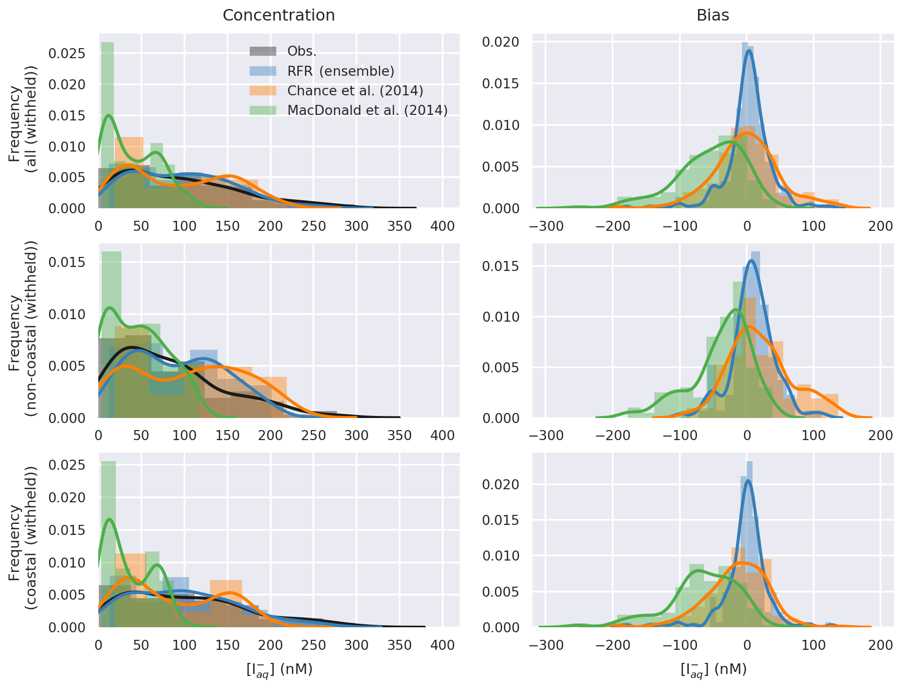
Figure 5Probability density function (bars) and Gaussian kernel density (lines) estimate of observations and predicted concentrations (left), and bias (right, model minus observations) in entire withheld dataset (upper, N=259), the withheld coastal dataset (middle, N=157), and the withheld non-coastal dataset (lower, N=102).
图 5整个保留数据集(上, N = 259 )(保留沿海数据集)中观测值和预测浓度(左)的概率密度函数(条形图)和高斯核密度(线)估计值和预测浓度(左)以及偏差(右,模型减去观测值) (中, N = 157 ),以及保留的非沿海数据集(下, N = 102 )。
The dataset selection error range, which shows the influence of the choice of how the dataset is split into training and withheld data on model prediction, is described in Sect. 3.2. Within the 20-member ensemble of different testing/withdrawn choices, the average variation in RMSE was 8.4 nM (5.9–11.02 nM), and in the range of average predicted values it was 6.1 nM (5.4–6.6 nM). This translates to a percentage error range of 13.9 %–36.3 % on the RMSE and 5.4 %–7.3 % on the average predicted value.
数据集选择误差范围,显示了数据集如何分割为训练数据和保留数据的选择对模型预测的影响,在第 1 节中进行了描述。 3.2 .在不同测试/撤回选择的 20 名成员中,RMSE 的平均变异为 8.4 nM (5.9–11.02 nM),在平均预测值范围内为 6.1 nM (5.4–6.6 nM)。这意味着 RMSE 的百分比误差范围为 13.9%–36.3%,平均预测值的百分比误差范围为 5.4%–7.3%。
The model selection error, which is the influence of the different independent variables used, is described in Sect. 3.2. The difference in the average prediction of the 10 members of the ensemble is 1.8 nM (with a range of average prediction from 96.0 to 97.8 nM), and the range of the difference in model performance is 3.9 nM (33.2–37.2 nM). As a percentage this model selection translates to a percentage uncertainty on the RMSE of 10.6 %–11.9 % and on the average of 1.8 %–1.9 %.
模型选择误差是所使用的不同自变量的影响,在第 4 节中进行了描述。 3.2 .集成的 10 个成员的平均预测差异为 1.8 nM(平均预测范围为 96.0 至 97.8 nM),模型性能差异范围为 3.9 nM(33.2-37.2 nM)。作为百分比,该模型选择转化为 RMSE 的百分比不确定性为 10.6%–11.9%,平均为 1.8%–1.9%。
The dataset selection and model selection compare to an error on the observations of ∼10 %. Uncertainty from dataset selection has a far greater effect on the prediction error than model selection. This is expected due to the small dataset size. The combined error in the prediction (dataset selection + model selection error) is either comparable to (7.2 %–9.2 % in terms of average prediction) or greater (24 %–48 % in terms of RMSE) than the observational error.
数据集选择和模型选择与观测值的误差相比约为10 %。数据集选择的不确定性对预测误差的影响比模型选择的影响大得多。由于数据集较小,这是预期的。预测中的组合误差(数据集选择 + 模型选择误差)与观测误差相当(就平均预测而言为 7.2%–9.2%),或者大于观测误差(就 RMSE 而言为 24%–48%)。
From this analysis we have shown that the new ensemble RFR model performs significantly better than those currently in the literature. We now turn to explore the predicted global distribution of sea-surface iodide using our ensemble model.
通过此分析,我们表明新的集成 RFR 模型的性能明显优于现有文献中的模型。我们现在转而使用我们的集合模型来探索海面碘化物的预测全球分布。
4.2 Global sea-surface iodide distribution
4.2全球海面碘化物分布
From the ensemble prediction system we calculate monthly global grids (
从集合预测系统中,我们计算每月的全球网格(
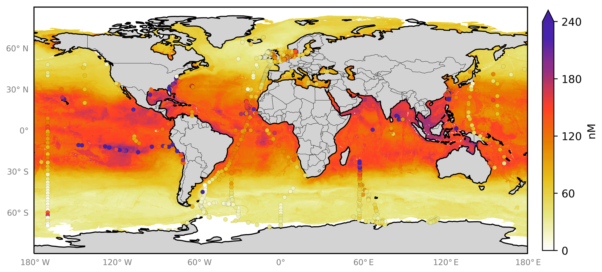
Figure 6Annual average predicted sea-surface iodide by the 10-member ensemble of models (RFR(Ensemble)), overlaid with iodide observations from Chance et al. (2019a) without outliers. Outliers are defined here as values greater than the third quartile plus 1.5 times the interquartile range (Frigge et al., 1989). Only locations that are entirely water are included in the spatial average. Earth raster and vector map data used are freely available from Natural Earth (http://www.naturalearthdata.com/, last access: 23 July 2019).
图 6由 10 人模型集合 (RFR(Ensemble)) 预测的年平均海面碘化物,与Chance 等人的碘化物观测结果重叠。 ( 2019 a )没有异常值。异常值在此定义为大于第三个四分位数加上 1.5 倍四分位距的值( Frigge 等, 1989 ) 。只有完全由水组成的位置才包含在空间平均值中。使用的地球栅格和矢量地图数据可从 Natural Earth 免费获取( http://www.naturalearthdata.com/ ,最后访问日期:2019 年 7 月 23 日)。
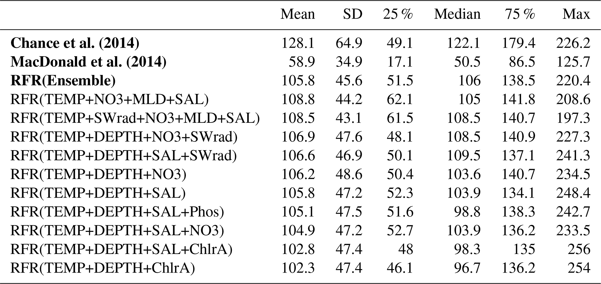
Summary statistics on the global predictions are shown in Table 4. These show that, as for comparisons at the observed locations (Sect. 4.1), the ensemble prediction is broadly in between the two existing parameters. The new ensemble model predicts a mean value of 106 nM (with members ranging from 102.3 to 108.8 nM), with predicted values from existing parameterisations ranging from 58.9 (MacDonald et al., 2014) to 128.1 nM (Chance et al., 2014).
全球预测的汇总统计数据如表4所示。这些表明,对于观测位置的比较(第4.1节),集合预测大致介于两个现有参数之间。新的集成模型预测平均值为 106 nM(成员范围为 102.3 至 108.8 nM),现有参数化的预测值范围为 58.9 ( MacDonald 等人, 2014 )至 128.1 nM ( Chance 等人, 2014 ) 。
Table 4Statistics on predicted global annual sea-surface values from new and existing parameters at a horizontal resolution of
表 4根据新参数和现有参数预测的全球年海面值的统计数据,水平分辨率为
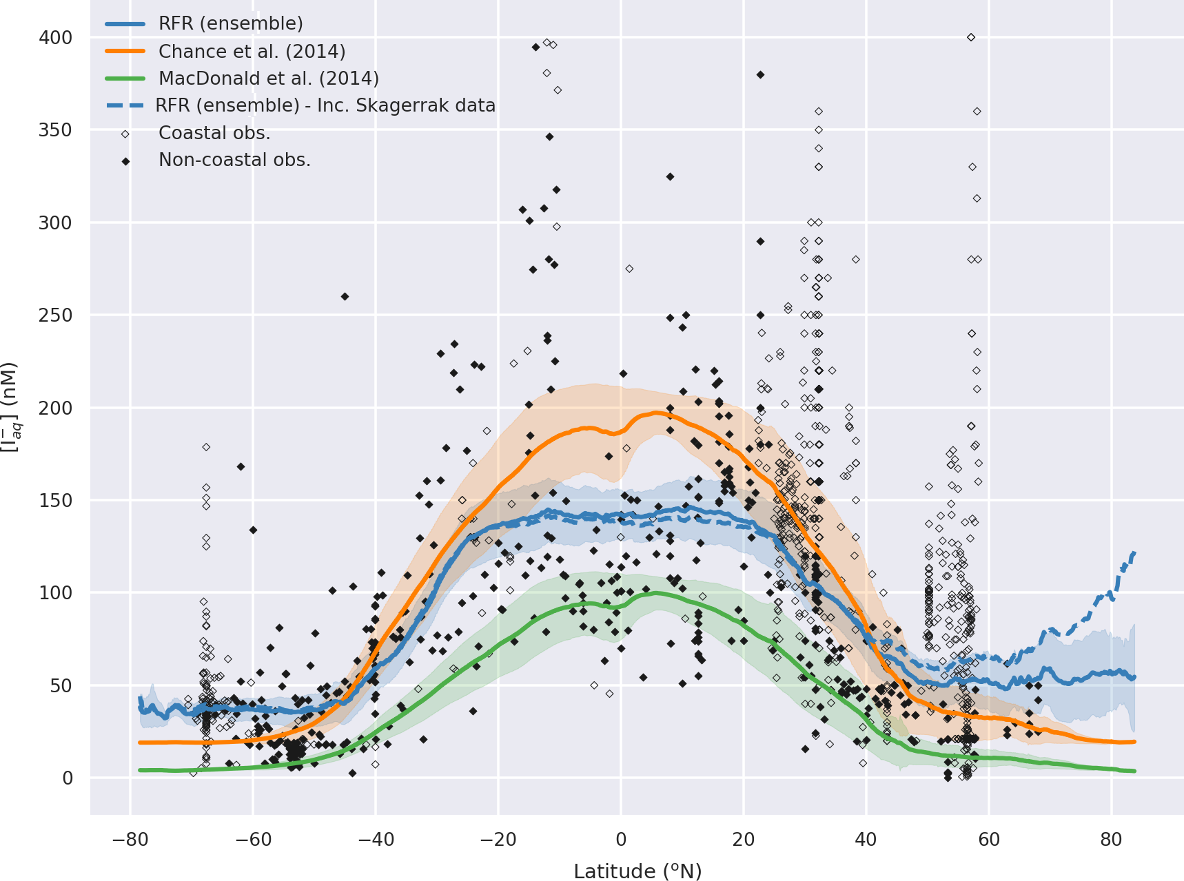
The annual latitudinal average of these fields, together with predictions from Chance et al. (2014) and MacDonald et al. (2014), and the observations are shown in Fig. 7. Far greater structure is seen compared to the two existing parameterisations (Fig. 7) due to the multivariate and non-parametric ensemble approach used here. All parameterisations capture the broad observed feature of decreasing iodide from lower to higher latitude. The new predicted values lie between Chance et al. (2014) and MacDonald et al. (2014) in the tropics; however, within the polar regions, the new prediction is significantly higher than both of the previous parameterisations. The lower concentrations in the predicted values from MacDonald et al. (2014) for most of the global sea surface are clear.
这些油田的年纬度平均值以及Chance 等人的预测。 ( 2014 )和麦克唐纳等人。 ( 2014 ) ,观察结果如图7所示。由于此处使用的多元和非参数集成方法,与两个现有参数化(图7 )相比,可以看到更大的结构。所有参数化都捕获了从低纬度到高纬度碘化物减少的广泛观察到的特征。新的预测值介于Chance 等人之间。 ( 2014 )和麦克唐纳等人。 ( 2014 )在热带地区;然而,在极地地区,新的预测明显高于之前的参数化。 MacDonald 等人的预测值中浓度较低。 ( 2014 )全球大部分海面都是晴朗的。
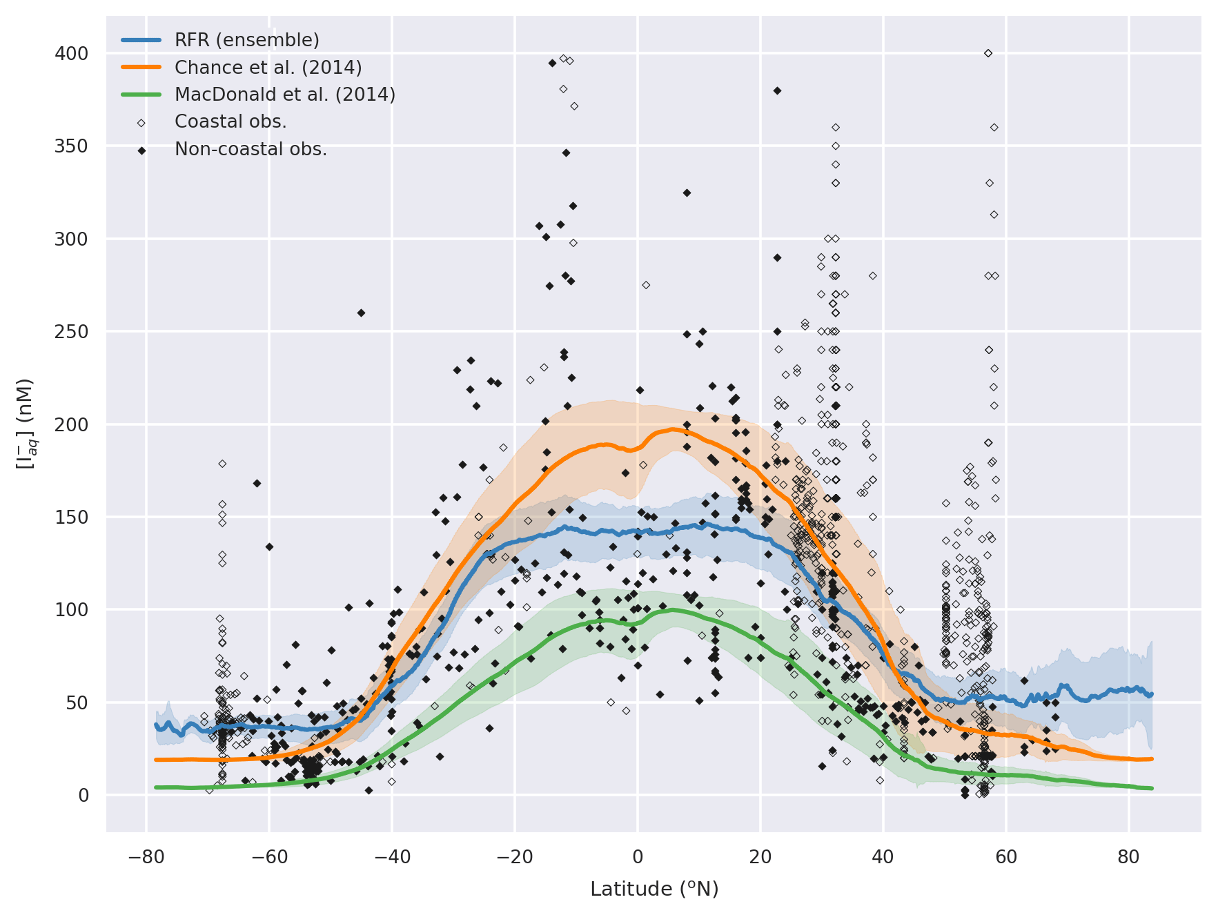
Figure 7Predicted annual average sea-surface iodide plotted against latitude (lines), overlaid with observed concentrations (diamonds). Solid lines give mean values and shaded regions give (±) the average standard deviation. The standard deviation is the monthly standard deviation across a latitude between all 10 ensemble members (RFR(Ensemble)) or within a single prediction for existing parameterisations (Chance et al., 2014; MacDonald et al., 2014). Filled diamonds show non-coastal observations and non-filled ones show coastal values. Extent of x axis is shown for grid boxes that are entirely water.
图 7根据纬度绘制的预测年平均海面碘化物(线),与观测到的浓度(菱形)重叠。实线给出平均值,阴影区域给出 ( ± ) 平均标准偏差。标准差是跨纬度所有 10 个集合成员 (RFR(Ensemble)) 或现有参数化的单个预测内的月标准差( Chance 等人, 2014 年; MacDonald 等人, 2014 年) 。填充的菱形显示非沿海观测值,未填充的菱形显示沿海值。显示完全由水组成的网格框的x轴范围。
The range of dataset error is found for the 20 models with different training data splits, as described in Sect. 3.2. This gives an uncertainty in the form of a average range in predicted global mean surface iodide for all of the multiple builds of ensemble members of 4.0 nM (2.8–5.0) compared to a annual mean prediction of 106 nM. This maximum and minimum of this range in predicted values can then be divided by the minimum and maximum predicted global mean surface iodide values (98 and 109.3 nM, respectively) to give percent range of 2.5 % to 5.1 %. This is lower than that calculated for the individual locations of observations (Sect. 4.1) due to large global areas being similar in chemical and physical regimes compared to the subset of sampled locations within the observations.
找到具有不同训练数据分割的 20 个模型的数据集误差范围,如第 2 节所述。 3.2 .这给出了所有多重构建的集合成员的预测全球平均表面碘化物平均范围为 4.0 nM (2.8–5.0) 的不确定性,而年平均预测为 106 nM。然后可以将该预测值范围的最大值和最小值除以预测的全球平均表面碘化物值的最小值和最大值(分别为 98 和 109.3 nM),得到 2.5% 至 5.1% 的百分比范围。这低于针对单个观测位置计算的值(第4.1节),因为与观测中采样位置的子集相比,大范围的全球区域在化学和物理状况方面相似。
The model selection error due to variability within ensembles' 10 members, generated with different independent variables, gives a global average surface concentration between 102.3 and 108.8 nM. This range in prediction gives a model selection error of 6.45 nM, which equates to 6.0 %–6.3 %. Like with the global uncertainty from dataset selection, the global value would be expected to be lower than the uncertainty at the specific locations of the observations (Sect. 4.1) due to the more homogeneous nature of the predicted areas. However, a greater variation is seen from different model predictions than within predictions for the observation locations. This highlights the importance of the different ancillary variables considered here and also therefore the strength gained from the ensemble approach taken here.
由于由不同自变量生成的集合 10 个成员内的变异性导致的模型选择误差给出了 102.3 至 108.8 nM 之间的全局平均表面浓度。此预测范围给出的模型选择误差为 6.45 nM,相当于 6.0%–6.3%。与数据集选择的全局不确定性一样,由于预测区域的更均匀性质,预计全局值将低于观测特定位置的不确定性(第4.1节)。然而,与观测位置的预测相比,不同模型的预测存在更大的差异。这凸显了此处考虑的不同辅助变量的重要性,以及从此处采用的集成方法中获得的力量。
Within members of the ensemble, variation is modest except for two ensemble members which diverge north of
在该群的成员中,除了两个群成员在北面发散之外,变化不大。
In addition to the three errors described above, we also attempt to gain an understanding of the spatial uncertainty in the 10-model ensemble prediction. We do this by calculating the differences in the predicted spatial fields from the 10 ensemble members. Figure 8 shows the monthly average of the standard deviation of the 10 model ensemble as a percentage of the annual mean of the ensemble prediction. This is also shown in absolute terms in the Appendix (Fig. A4). Relative uncertainties are largest at the poles where predicted concentrations are lowest and where (at least in the Northern Hemisphere) very few observations are available to constrain the system. The southern oceans show an distinct pattern, where values close to coastal Antarctica appear well constrained but values further north appear poorly constrained.
除了上述三个错误之外,我们还尝试了解 10 模型集成预测中的空间不确定性。我们通过计算 10 个集合成员的预测空间场的差异来实现这一点。图8显示了 10 个模型集合的标准差的月平均值占集合预测年平均值的百分比。这也以绝对值的形式显示在附录中(图A4 )。两极的相对不确定性最大,那里的预测浓度最低,并且(至少在北半球)可用于约束系统的观测数据非常少。南部海洋显示出一种独特的模式,其中靠近南极洲沿海的值似乎受到很好的约束,但更北的值似乎受到很弱的约束。
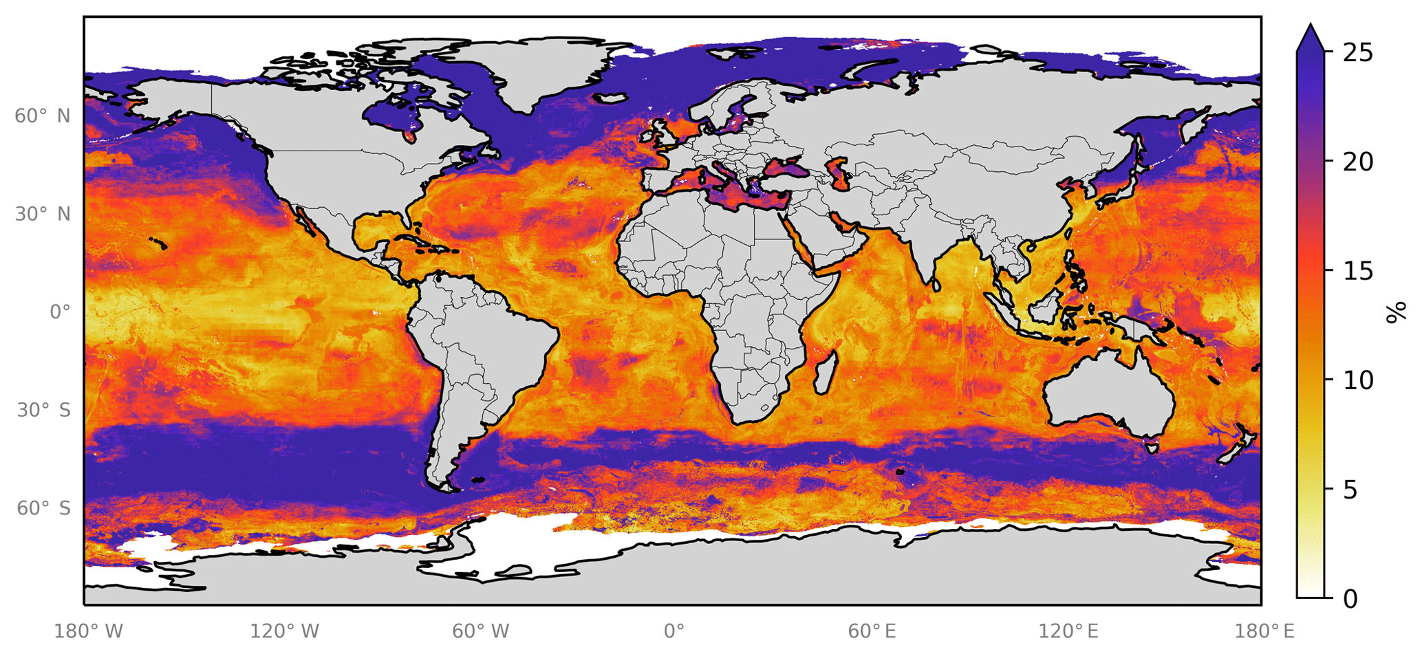
Figure 8Annual average spatial percent uncertainty in predicted sea-surface iodide for the ensemble of models. Percent spatial uncertainty was calculated as the standard deviation in monthly average values for all models, divided by the annual mean. Values are limited to 25 % for contrast, but the maximum plotted value is 77 % in the northern high latitudes. Only locations that are entirely water are included in the spatial average. Earth raster and vector map data used are freely available from Natural Earth (http://www.naturalearthdata.com/, last access: 23 July 2019).
图 8模型集合预测的海面碘化物的年平均空间百分比不确定性。空间不确定性百分比计算为所有模型月平均值的标准差除以年平均值。对比度值限制为 25%,但在北部高纬度地区绘制的最大值为 77%。只有完全由水组成的位置才包含在空间平均值中。使用的地球栅格和矢量地图数据可从 Natural Earth 免费获取( http://www.naturalearthdata.com/ ,最后访问日期:2019 年 7 月 23 日)。
5数据可用性
The monthly ensemble mean and standard deviation between ensemble members for the main prediction presented here (RFR(Ensemble)), along with the individual ensemble members, are archived at the United Kingdom's Centre for Environmental Data Analysis (CEDA) as monthly files in NetCDF-4 format (Sherwen et al., 2019; https://doi.org/10/gfv5v3). To enable use in atmospheric and oceanic models, we have additionally bilinearly re-gridded the outputted fields onto common model grids (Appendix Table A4) using the open-source Python xESMF package (Zhuang, 2018). Values are provided for all locations globally and indices of land–water–ice cover are provided to allow data users to choose how to treat locations where water meets ice or land; however, we would not recommend the use of predicted values where ice or land are present. We recommended use of the standard output provided but have also provided the predictions made by the model with the Skagerrak dataset (Truesdale et al., 2003) included (which was excluded from the analysis presented here, as discussed further in Appendix Sect. A1).
这里介绍的主要预测的集合成员之间的每月集合平均值和标准差 (RFR(Ensemble)) 以及各个集合成员,均作为 NetCDF 中的每月文件存档在英国环境数据分析中心 (CEDA) - 4 格式( Sherwen 等人, 2019 ; https://doi.org/10/gfv5v3 )。为了能够在大气和海洋模型中使用,我们还使用开源 Python xESMF 包( Zhang , 2018 )将输出字段双线性重新网格化到通用模型网格上(附录表A4 )。提供了全球所有地点的数值,并提供了土地-水-冰覆盖指数,以便数据用户选择如何处理水与冰或土地相遇的地点;然而,我们不建议在存在冰或陆地的地方使用预测值。我们建议使用所提供的标准输出,但也提供了包含 Skagerrak 数据集( Truesdale 等人, 2003 )的模型所做的预测(已从此处提供的分析中排除,如附录A1节中进一步讨论) 。
Ancillary data extracted for observation locations and used to predict spatial fields are available from sources stated in Table 1. Iodide observations are described by Chance et al. (2019a) and made available by the British Oceanographic Data Centre (BODC, Chance et al., 2019b; https://doi.org/10/czhx).
为观测位置提取并用于预测空间场的辅助数据可从表1中所述的来源获得。 Chance 等人描述了碘化物的观察结果。 ( 2019 a )并由英国海洋学数据中心提供(BODC、 Chance 等人, 2019 b ; https://doi.org/10/czhx )。
6代码可用性
Data analysis and processing used open-source Python packages, including Pandas (McKinney, 2010), Xarray (Hoyer and Hamman, 2017), and Scikit-learn (Pedregosa et al., 2011). Spatial re-gridding used the xESMF package (Zhuang, 2018). Plots presented here were created using the Matplotlib (Hunter, 2007), Seaborn (Waskom et al., 2017), and Cartopy (Elson et al., 2018) Python packages. The specific routines used for this work are archived within the sparse2spatial package (Sherwen, 2019), with the exception of the decision tree figures (Figs. 3 and A5), which were made using the TreeSurgeon package (Ellis and Sherwen, 2019).
数据分析和处理使用开源Python包,包括Pandas ( McKinney , 2010 ) 、Xarray ( Hoyer和Hamman , 2017 )和Scikit-learn ( Pedregosa等人, 2011 ) 。空间重新网格化使用了xESMF包( Zhang , 2018 ) 。此处展示的绘图是使用 Matplotlib ( Hunter , 2007 ) 、Seaborn ( Waskom 等人, 2017 )和 Cartopy ( Elson 等人, 2018 ) Python 包创建的。这项工作使用的具体例程存档在稀疏2spatial包中( Sherwen , 2019 ) ,但决策树图(图3和A5 )除外,它是使用TreeSurgeon包制作的( Ellis和Sherwen , 2019 ) 。
7讨论与结论
Here we have explored the ability of an algorithmic approach combined with various physical and chemical variables to predict sea-surface iodide, without aiming to represent the biogeochemical or abiotic processes occurring. This approach instead gives a data-driven best guess at concentrations and an ability to quantify where the greatest uncertainty lies. However, certain features such as prediction of an apparent relationship between ocean bathymetry and sea-surface iodide concentrations, where the ocean is very deep (e.g. over the Mid-Atlantic Ridge), are unlikely to have a plausible physical explanation (Fig. 6).
在这里,我们探索了算法方法与各种物理和化学变量相结合来预测海面碘化物的能力,而不是为了代表发生的生物地球化学或非生物过程。相反,这种方法提供了数据驱动的浓度最佳猜测,并能够量化最大不确定性所在。然而,某些特征,例如海洋深部测量与海面碘化物浓度之间明显关系的预测,在海洋很深的地方(例如大西洋中脊上方),不太可能有合理的物理解释(图6 ) 。
The new spatial prediction presented here differs from what has been used previously in atmospheric models (e.g. Chance et al., 2014; MacDonald et al., 2014). Although the average value lies between these parameterisations, the prediction is closest to that from Chance et al. (2014) even with larger values found at higher latitudes. As most atmospheric models have used the iodide parameterisation from MacDonald et al. (2014) to calculate ocean iodine emissions (Appendix Table A1), a higher emission would therefore now be expected. This would result in larger decreases in tropospheric ozone burden than previously suggested (Sherwen et al., 2016a). A higher iodide sea-surface concentration would also result in a greater calculated ozone deposition (Ganzeveld et al., 2009; Luhar et al., 2017; Sarwar et al., 2016).
这里提出的新空间预测与以前在大气模型中使用的预测不同(例如Chance 等人, 2014 年; MacDonald 等人, 2014 年)。尽管平均值位于这些参数化之间,但预测最接近Chance 等人的预测。 ( 2014 )即使在高纬度地区发现了更大的值。由于大多数大气模型都使用了MacDonald 等人的碘化物参数化。 ( 2014 )计算海洋碘排放量(附录表A1 ),因此现在预计排放量会更高。这将导致对流层臭氧负担比之前建议的减少幅度更大( Sherwen 等, 2016a ) 。海面碘化物浓度越高,计算得出的臭氧沉积量也越大( Ganzeveld 等人, 2009 年; Luhar 等人, 2017 年; Sarwar 等人, 2016 年) 。
We have calculated the errors in sea-surface iodide concentrations at observational locations due to the dataset selection of 13.9 %–36.3 % and due to the model selection of 1.8 %–1.9 % (Sect. 4.1 and 4.2). These error estimates can be compared to an approximated error in the observations of ∼10 % (Chance et al., 2019a). Considering that the average predicted global concentration here is 106 nM (Sect. 4.2), these errors are notable. The greatest driver in error is the dataset selection. More observations, and particularly observations representative of under-sampled areas (e.g. Arctic) and seasons, will be required to reduce this error. The error caused by dataset selection is also reduced when the predictions are considered spatially over the global sea surface.
由于数据集选择为 13.9%–36.3%,模型选择为 1.8%–1.9%,我们计算了观测地点海面碘化物浓度的误差(第4.1和4.2节)。这些误差估计可以与∼10 % 的观测值的近似误差进行比较( Chance 等人, 2019 年a ) 。考虑到这里的平均预测全局浓度为 106 nM(第4.2节),这些错误是值得注意的。最大的错误驱动因素是数据集的选择。需要更多的观测,特别是代表采样不足的地区(例如北极)和季节的观测,以减少这种误差。当在全球海面空间上考虑预测时,由数据集选择引起的误差也会减少。
The choice of the algorithm used here is subjective and numerous other options are available. The random forest regressor was chosen due to its appropriateness for the continuous regression task performed here, its relatively cheap computation cost, and its interpretability. Considering the greatest uncertainty is driven by the paucity and sparsity of observations, using more complex techniques would not be expected to yield particularly different or drastically better results, considering other trade-offs.
这里使用的算法的选择是主观的,并且还有许多其他选项可用。选择随机森林回归器是因为它适合此处执行的连续回归任务、其相对便宜的计算成本及其可解释性。考虑到最大的不确定性是由观测的缺乏和稀疏造成的,考虑到其他权衡,使用更复杂的技术预计不会产生特别不同或明显更好的结果。
We have developed a new way to build a spatially and temporally resolved dataset from a spatially and temporally sparse input of observations. This has allowed for the use of more observations than traditional approaches, which is particularly important with a paucity of data. This approach has demonstrated a large improvement in skill in terms of capturing observations compared to the existing parameterisations in use. It captures the pattern of decreasing iodide with higher latitude seen in the observations, as well as the greater spatial variation seen in the observations.
我们开发了一种新方法,可以根据空间和时间稀疏的观测输入构建空间和时间解析的数据集。与传统方法相比,这允许使用更多的观察结果,这在数据匮乏的情况下尤为重要。与现有使用的参数化相比,这种方法在捕获观察方面的技能有了很大的提高。它捕获了观测中观察到的随着纬度越高碘化物减少的模式,以及观察中观察到的更大的空间变化。
A1 Removed Skagerrak dataset
A1删除了 Skagerrak 数据集
Ideally with sparse datasets as much data as possible would be included for training the regression models used. If a feature in the data is different enough to the rest of the dataset and not sufficiently represented for the regressor model to characterise it, then it has the potential to introduce a large dataset error (see Sect. 3.2 for details). This was shown when the iodide values above the outlier threshold were included (Sect. 3.2). There could be many other effects of including data that are significantly different to the rest of the dataset.
理想情况下,对于稀疏数据集,将包含尽可能多的数据来训练所使用的回归模型。如果数据中的某个特征与数据集的其余部分有足够的差异,并且没有充分代表回归模型来表征它,那么它有可能引入大的数据集错误(详细信息请参见第3.2节)。当碘化物值高于离群值阈值时,就会出现这种情况(第3.2节)。包含与数据集其他部分显着不同的数据可能会产生许多其他影响。
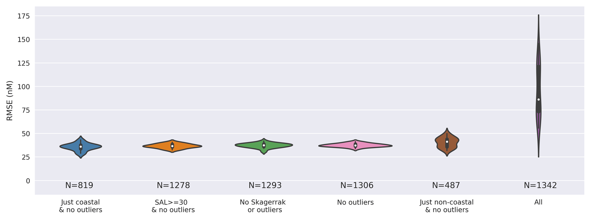
Figure A1Combined kernel density and violin plots showing the distribution of the root mean square error (RMSE) for 20 different models built from 20 different pseudo-random initialisations for a different selection of the dataset as described in Table 2 and Sect.3.2. Models built using the whole dataset (“all”), including outliers, show a significantly higher RMSE due to observations with higher iodide concentrations. The model used here includes ancillary variables of temperature, depth, and salinity which were thought to intuitively give a reasonable result.
图 A1组合核密度和小提琴图显示了 20 个不同模型的均方根误差 (RMSE) 分布,这些模型是根据表2和第 2 节中所述的不同数据集选择的 20 个不同伪随机初始化构建的。 3.2 .由于碘化物浓度较高,使用整个数据集(“全部”)(包括异常值)构建的模型显示出明显较高的 RMSE。这里使用的模型包括温度、深度和盐度等辅助变量,这些变量被认为可以直观地给出合理的结果。
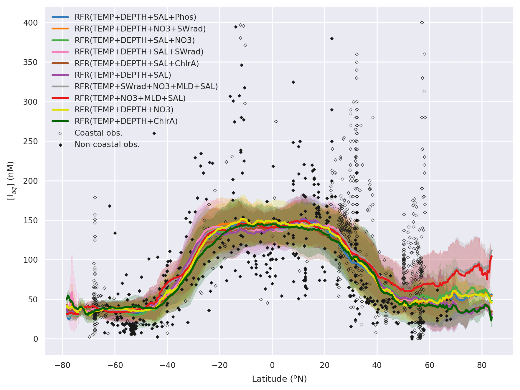
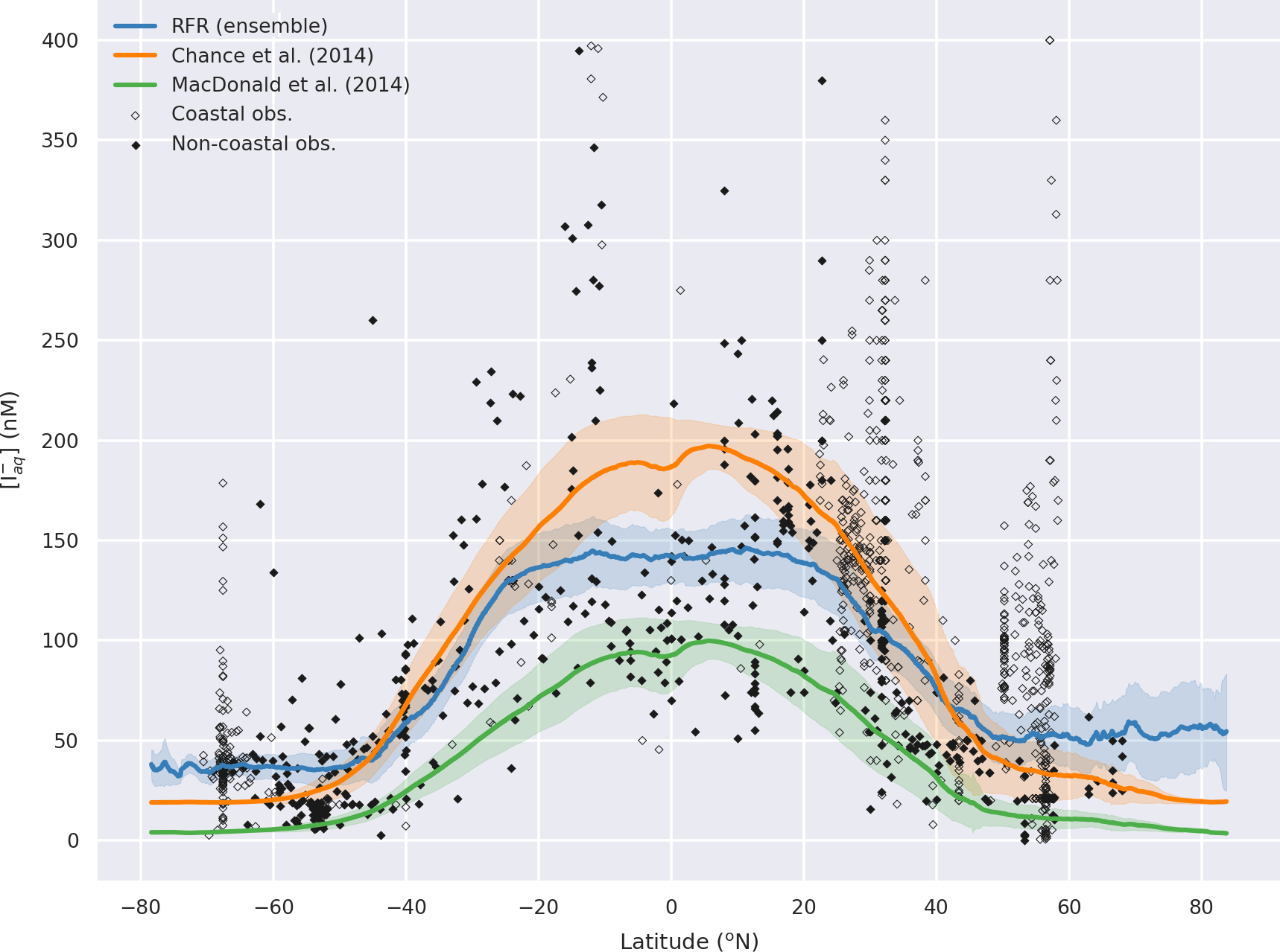
Figure A2Predicted global sea-surface iodide for all ensemble members plotted against latitude, overlaid with observed concentrations. Shaded regions give (±) the average standard deviation for a given latitude. The standard deviation is the monthly standard deviation for a single ensemble members (RFR(Ensemble)) or within a single prediction for existing parameterisations (Chance et al., 2014; MacDonald et al., 2014). Filled diamonds show non-coastal observations and unfilled ones show coastal values. Extent of x axis is shown for grid boxes that are entirely water.
图 A2根据纬度绘制所有集合成员的预测全球海面碘化物,并与观测到的浓度重叠。阴影区域给出给定纬度的平均标准偏差 ( ± )。标准差是单个集成成员 (RFR(Ensemble)) 或现有参数化的单个预测内的月标准差( Chance et al. , 2014 ; MacDonald et al. , 2014 ) 。填充的菱形显示非海岸观测值,未填充的菱形显示海岸值。显示完全由水组成的网格框的x轴范围。

Figure A3Percentage difference in monthly sea-surface iodide from the annual mean field predicted by the 10-model member ensemble. Only locations that are entirely water are included. Earth raster and vector map data used are freely available from Natural Earth (http://www.naturalearthdata.com/, last access: 23 July 2019).
图 A3月海面碘化物与 10 模型成员集合预测的年平均场的百分比差异。仅包括完全由水组成的位置。使用的地球栅格和矢量地图数据可从 Natural Earth 免费获取( http://www.naturalearthdata.com/ ,最后访问日期:2019 年 7 月 23 日)。
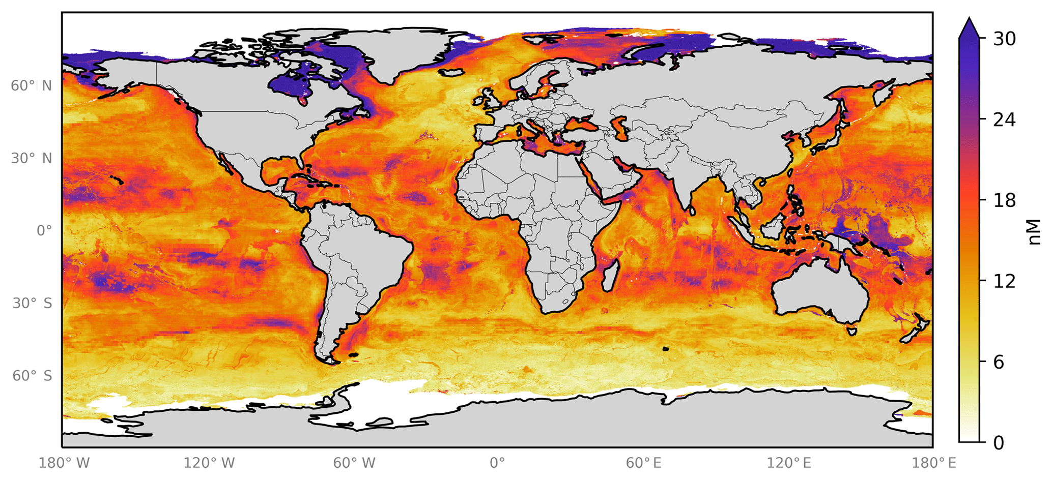
Figure A4Annual average spatial uncertainty in predicted sea-surface iodide for the ensemble of 10 models. Spatial variation was calculated as the standard deviation in monthly average values for all models. Values are limited to 30 nM for contrast, and the maximum value plotted is 52 nM in the northern high latitudes. Only locations that are entirely water are included in spatial the average. Earth raster and vector map data used are freely available from Natural Earth (http://www.naturalearthdata.com/, last access: 23 July 2019).
图 A4 10 个模型集合预测的海面碘化物的年平均空间不确定性。空间变异计算为所有模型月平均值的标准差。为了对比,值限制为 30 nM,在北部高纬度地区绘制的最大值为 52 nM。只有完全由水组成的位置才包含在空间平均值中。使用的地球栅格和矢量地图数据可从 Natural Earth 免费获取( http://www.naturalearthdata.com/ ,上次访问日期:2019 年 7 月 23 日)。

Figure A5Representation of all forests within the 10-member ensemble (also shown as thumbnails in Fig. 3c). The branches are coloured by percentage of each variable that drives the decision at a given node. The thickness of branches gives the average throughput of the dataset through a given node. Variable names are coloured as per the following coloured text: temperature (blue, ∘C), depth (orange,metres), chlorophyll a (green, mg m−3), salinity (pink, PSU), nitrate (brown, µg m−3), mixed layer depth (MLD; purple, metres), phosphate (red, µg m−3), and shortwave radiation (grey, W m−2)
图 A5 10 成员集合中所有森林的表示(也在图3 c 中显示为缩略图)。分支按驱动给定节点决策的每个变量的百分比进行着色。分支的厚度给出了通过给定节点的数据集的平均吞吐量。变量名称按照以下彩色文本着色:温度(蓝色, ∘ C)、深度(橙色,米)、叶绿素a (绿色,mg m −3 )、盐度(粉红色,PSU)、硝酸盐(棕色, μg m −3 )、混合层深度(MLD;紫色,米)、磷酸盐(红色, μg m −3 )和短波辐射(灰色,W m −2 )

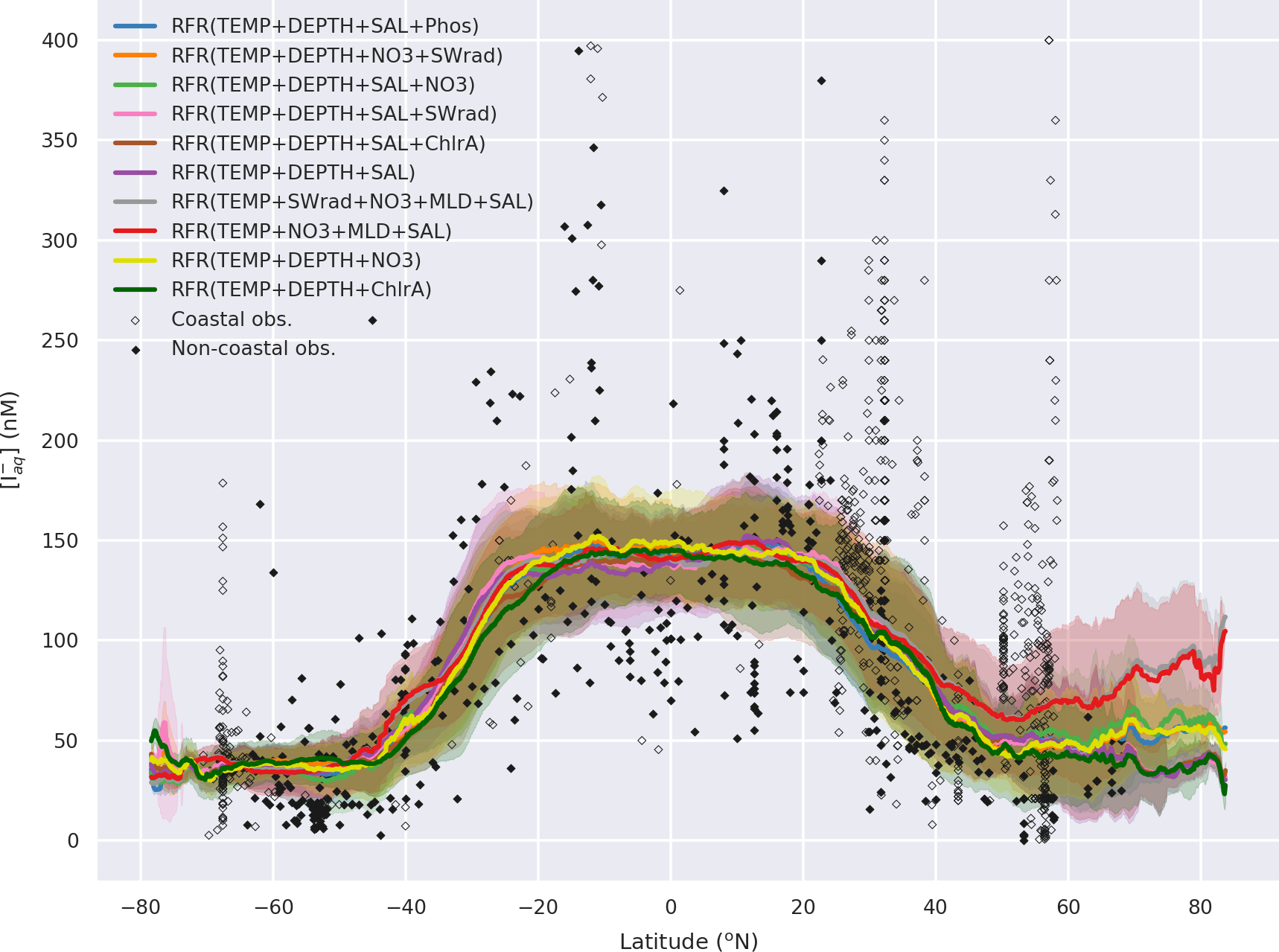
Figure A6Predicted latitudinal average sea-surface iodide plotted against latitude, overlaid with observed concentrations. Figure is equivalent to Fig. 7, but the dashed line shows the prediction including data from the Skagerrak strait (Truesdale et al., 2003). Solid lines give mean values and shaded regions give ± the average standard deviation. For the ensemble the standard deviation is the monthly standard deviation within all ensemble members. Filled diamonds show non-coastal observations and unfilled ones show coastal values. Extent of x axis is shown for grid boxes that are entirely water.
图 A6根据纬度绘制预测的纬度平均海面碘化物,并与观测到的浓度重叠。该图与图7相同,但虚线显示了包含斯卡格拉克海峡数据的预测( Truesdale 等, 2003 ) 。实线给出平均值,阴影区域给出±平均标准差。对于整体而言,标准偏差是所有整体成员内的每月标准偏差。填充的菱形显示非海岸观测值,未填充的菱形显示海岸值。显示完全由水组成的网格框的x轴范围。
The data from the Skagerrak strait (Truesdale et al., 2003), which are included in the (Chance et al., 2019a) compilation of iodide data, were excluded from this analysis. This is because, upon inclusion, high iodide at high latitudes (
来自斯卡格拉克海峡的数据( Truesdale 等人, 2003 年)包含在碘化物数据汇编( Chance 等人, 2019 年a )中,但被排除在本次分析之外。这是因为,在纳入后,高纬度地区的碘化物含量较高(
The Skagerrak strait data (Truesdale et al., 2003) are also from a region where the observed ancillary variables compare poorly with those extracted from ancillary datasets. Observed salinity is between 24.0 and 33.5 PSU, whereas the climatological value is 31.7 to 35.8 PSU. This equates to a bias of the climatology versus the in situ observations of up to 9.6 PSU or 40 %. The Skagerrak is biogeochemically different from the Arctic, and its large influence on predicted values in the Arctic may arise simply from its latitudinal proximity, given the lack of observations from the regions themselves.
斯卡格拉克海峡数据( Truesdale 等, 2003 )也来自一个区域,该区域观测到的辅助变量与从辅助数据集中提取的变量相比效果较差。观测到的盐度在 24.0 至 33.5 PSU 之间,而气候值在 31.7 至 35.8 PSU 之间。这相当于气候学与现场观测的偏差高达 9.6 PSU 或 40%。斯卡格拉克地区在生物地球化学方面与北极不同,鉴于缺乏对该地区本身的观测,其对北极预测值的巨大影响可能仅仅是由于其纬度上的接近性。
张等人。 (2004)哦等人。 (2008)科尔曼等人。 (2010)Ganzeveld 等人。 (2009)普拉多斯-罗曼等人。 (2015) 赛兹-洛佩兹等人。 (2014)甘特等人。 (2017) 萨瓦尔等人。 (2016, 2015)Sherwen 等人。 (2016a)Sherwen 等人。 (2016b, c, 2017a, b)Luhar 等人。 (2017、2018)
Table A1Summary of sea-surface iodide parameterisations in global and regional atmospheric models.
表 A1全球和区域大气模型中海面碘化物参数化总结。
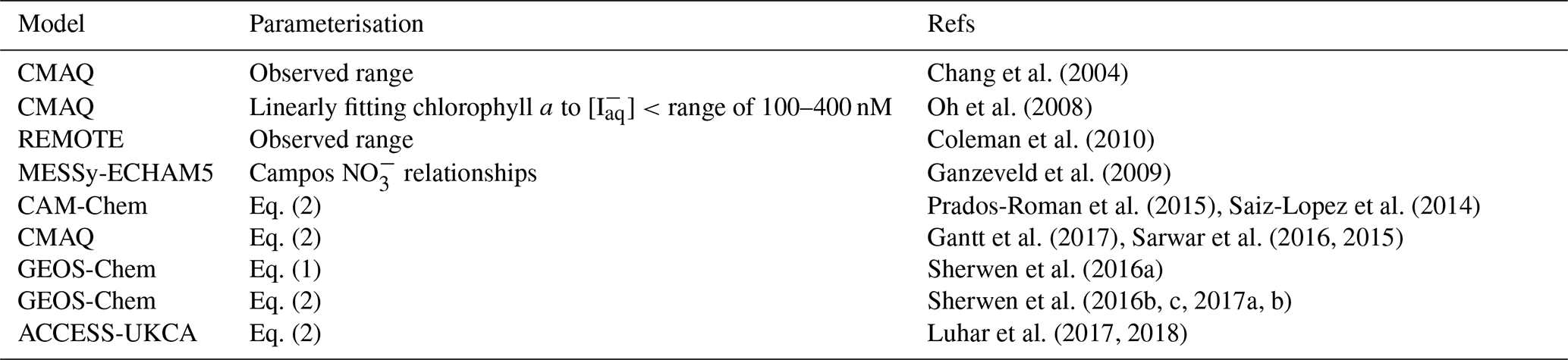
Table A2Statistics on observations and predicted values from the new ensemble and existing parameterisations at locations of observations. Root mean square error (RMSE) is shown against the withheld data and the entire dataset of observations. Ensemble members, ensemble prediction (RFR(Ensemble)), and existing parameterisations shown in bold. Values are shown for all 38 models built, including those not included in the ensemble.
表 A2新集合的观测值和预测值以及观测位置现有参数化的统计数据。显示针对保留数据和整个观测数据集的均方根误差 (RMSE)。集成成员、集成预测 (RFR(Ensemble)) 和现有参数化以粗体显示。显示了所有 38 个已构建模型的值,包括未包含在整体中的模型。
机会等人。 (2014) 麦克唐纳等人。 (2014)
Table A3Statistics on observations and predicted values by ensemble and existing parameterisations at locations of observations but just for the withheld dataset locations. Table 3 shows the values for both the withheld and entire dataset.
表 A3观测值和预测值的统计数据以及观测位置的现有参数化,但仅适用于保留的数据集位置。表3显示了保留数据集和整个数据集的值。
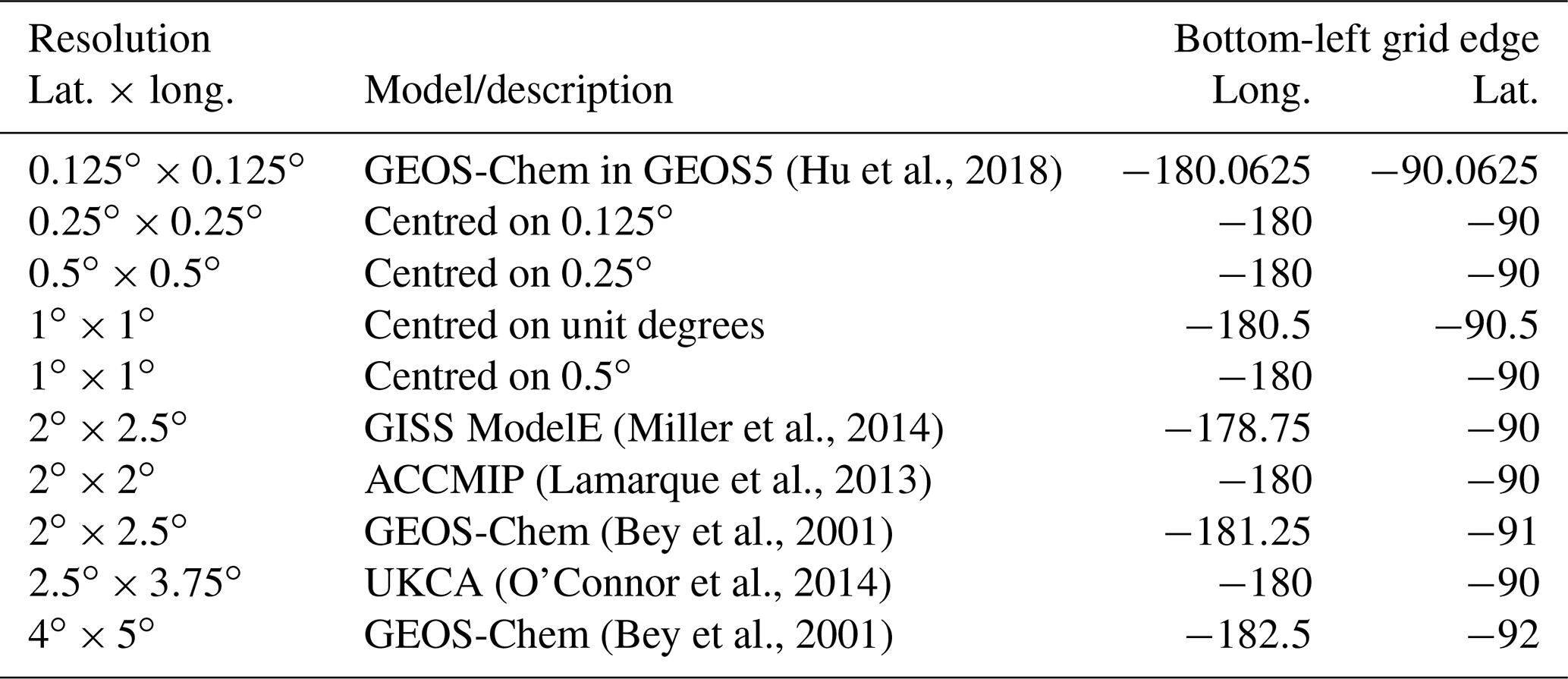
(Hu 等人,2018)(Miller 等人,2014)(Lamarque 等人,2013)(Bey 等人,2001)(O'Connor 等人,2014)(Bey 等人,2001)
Table A4Spatial and temporal resolutions of global monthly iodide fields available for download from the United Kingdom's Centre from Environmental Data Analysis (Sherwen et al., 2019; https://doi.org/10/gfv5v3). Re-gridding was performed in Python using the open-source xESMF package (Zhuang, 2018).
表 A4全球每月碘化物场的空间和时间分辨率可从英国环境数据分析中心下载( Sherwen 等人, 2019 年; https://doi.org/10/gfv5v3 )。使用开源 xESMF 包在 Python 中执行重新网格化( Zhang , 2018 ) 。
Latitudes less than
纬度小于
The area this dataset is sampling in is also unusual in the Chance et al. (2019a) compilation due to its estuarine nature. However, this cannot entirely explain its behaviour as their are other estuarine datasets included (such as those from around the Chesapeake Bay, Luther and Cole, 1988; Wong and Cheng, 1998, 2008) which do not cause the same issue.
该数据集采样的区域在Chance 等人中也很不寻常。 ( 2019 a )由于其河口性质而编制。然而,这不能完全解释其行为,因为它们包含的其他河口数据集(例如来自切萨皮克湾周围的数据集, Luther and Cole , 1988 ; Wong and Cheng , 1998,2008 )不会引起同样的问题。
As the feature of high predicted Arctic iodide is driven by a single dataset of 19 samples (of which 4 would be removed as outliers) from a different region, it is highly uncertain. Not only do the in situ salinity observations compare poorly to the extracted ancillary ones, but the location itself represents a heterogeneity within the Chance et al. (2019b) compilation as it has relatively high observed iodide concentrations. It was therefore omitted from the analysis presented within this paper. However results with this dataset are included in the shared data outputs. It is hoped that further observations
由于高预测北极碘化物的特征是由来自不同区域的 19 个样本(其中 4 个将作为异常值去除)的单个数据集驱动的,因此具有高度不确定性。不仅原位盐度观测结果与提取的辅助观测结果相比较差,而且该位置本身也代表了 Chance 等人的异质性。 (2019b) 编译,因为观察到的碘化物浓度相对较高。因此,本文的分析中省略了它。然而,该数据集的结果包含在共享数据输出中。希望进一步观察
LJC, MJE, and TS conceived the work. TS developed the code, built the models, and performed the analysis. DE and TS wrote the code to make Fig. 3 and Appendix Fig. A5. TS wrote the paper with contributions from RJC, MJE, LT, and LJC.
LJC、MJE 和 TS 构思了这项工作。 TS 开发代码、构建模型并进行分析。 DE和TS编写了代码来制作图3和附录图A5。 TS 在 RJC、MJE、LT 和 LJC 的贡献下撰写了这篇论文。
The authors declare that they have no conflict of interest.
作者声明他们没有利益冲突。
We all thank those who have provided their published and unpublished data to the Chance et al. (2019a) dataset and the British Oceanographic Data Centre (BODC) for hosting this, as well as all support staff involved.
我们都感谢那些向Chance 等人提供已发表和未发表数据的人。 ( 2019 a )数据集和托管该数据集的英国海洋数据中心 (BODC) 以及所有相关支持人员。
We gratefully acknowledge those who have worked to compile and make available the ancillary datasets used here (Table 1). These include the World Ocean Atlas (WOA), Ocean Biology Processing Group (OBPG) at NASA's Goddard Space Flight Center, and the General Bathymetric Chart of the Oceans (GEBCO) teams.
我们衷心感谢那些致力于编译和提供此处使用的辅助数据集的人们(表1 )。其中包括世界海洋地图集 (WOA)、美国宇航局戈达德太空飞行中心的海洋生物处理小组 (OBPG) 和通用海洋测深图 (GEBCO) 团队。
We thank Tim Jickells, Peter Liss, David Stevens, and Martin Wadley for their useful conversations on and comments about this work.
我们感谢 Tim Jickells、Peter Liss、David Stevens 和 Martin Wadley 对这项工作进行的有益的对话和评论。
We gratefully acknowledge funding from Natural Environment Research Council (NERC) through grants “Iodide in the ocean: distribution and impact on iodine flux and ozone loss” (NE/N009983/1) and “Big data for atmospheric chemistry and composition: Understanding the Science (BACCHUS)” (NE/L01291X/1).
我们非常感谢自然环境研究委员会 (NERC) 通过赠款“海洋中的碘化物:分布及其对碘通量和臭氧损失的影响”(NE/N009983/1) 和“大气化学和成分的大数据:了解科学”提供的资助(酒神)”(NE/L01291X/1)。
This research has been supported by the Natural Environment Research Council grants “Iodide in
the ocean: distribution and impact on iodine flux and ozone
loss” (grant no. NE/N009983/1) and “Big data for atmospheric chemistry and composition: Understanding the Science (BACCHUS)” (grant no. NE/L01291X/1).
这项研究得到了自然环境研究委员会的资助“海洋中的碘化物:分布及其对碘通量和臭氧损失的影响”(资助号:NE/N009983/1)和“大气化学和成分的大数据:了解科学(巴克斯)”(授权号:NE/L01291X/1)。
This paper was edited by Scott Stevens and reviewed by Peer Johannes Nowack and Laurens Ganzeveld.
本文由 Scott Stevens 编辑,并由 Peer Johannes Nowack 和 Laurens Ganzeveld 审阅。
Becker, J. J., Sandwell, D. T., Smith, W. H. F., Braud, J., Binder, B., Depner,
J., Fabre, D., Factor, J., Ingalls, S., Kim, S.-H., Ladner, R., Marks, K.,
Nelson, S., Pharaoh, A., Trimmer, R., Rosenberg, J. V., Wallace, G., and
Weatherall, P.: Global Bathymetry and Elevation Data at 30 Arc Seconds
Resolution: SRTM30_PLUS, Mar. Geod., 32, 355–371,
https://doi.org/10.1080/01490410903297766, 2009. a
贝克尔,J.J.,桑德韦尔,D.T.,史密斯,WH F.,布劳德,J.,宾德,B.,德普纳,
J.,法布尔,D.,因素,J.,英格尔斯,S.,金,S.-H.,拉德纳,R.,马克斯,K.,
纳尔逊,S.,法老,A.,特里默,R.,罗森伯格,J.V.,华莱士,G.,和
Weatherall, P.:30 角秒的全球测深和高程数据
分辨率:SRTM30_PLUS,三月地理,32, 355–371,
https://doi.org/10.1080/01490410903297766,2009年。
Behrenfeld, M. J. and Falkowski, P. G.: Photosynthetic rates derived from
satellite-based chlorophyll concentration, Limnol. Oceanogr., 42,
1–20, https://doi.org/10.4319/lo.1997.42.1.0001,
1997. a
Behrenfeld, MJ 和 Falkowski, PG:根据卫星叶绿素浓度 Limnol 得出的光合速率。 Oceanogr.,42, 1–20, https://doi.org/10.4319/lo.1997.42.1.0001,1997年。
Bey, I., Jacob, D. J., Yantosca, R. M., Logan, J. A., Field, B. D., Fiore,
A. M., Li, Q., Liu, H. Y., Mickley, L. J., and Schultz, M. G.: Global
modeling of tropospheric chemistry with assimilated meteorology: Model
description and evaluation, J. Geophys. Res., 106, 23073–23095,
https://doi.org/10.1029/2001JD000807, 2001. a, b
Bey, I.、Jacob, D.J.、Yantosca, R.M.、Logan, J.A.、Field, B.D.、Fiore,
A. M.、Li, Q.、Liu, H. Y.、Mickley, L. J. 和 Schultz, M. G.:全球
利用同化气象学对对流层化学进行建模:模型
描述和评估,J. Geophys。论文,106, 23073–23095,
https://doi.org/10.1029/2001JD000807,2001.a,b
Breiman, L.: Random forests, Mach. Learn., 45, 5–32, 2001. a, b, c, d
Breiman, L.:随机森林,马赫。学习。, 45, 5–32, 2001. a , b , c , d
Campos, M., Farrenkopf, A., Jickells, T., and Luther, G.: A comparison of
dissolved iodine cycling at the Bermuda Atlantic Time-series Station and
Hawaii Ocean Time-series Station, Deep Sea Res. Pt. II, 43, 455–466, https://doi.org/10.1016/0967-0645(95)00100-X,
1996. a
Campos, M.、Farrenkopf, A.、Jickells, T. 和 Luther, G.:百慕大大西洋时间序列站和夏威夷海洋时间序列站溶解碘循环的比较,深海研究中心。铂。 II,43, 455–466, https://doi.org/10.1016/0967-0645(95 )00100- X ,1996 年。
Carpenter, L. J., MacDonald, S. M., Shaw, M. D., Kumar, R., Saunders, R. W.,
Parthipan, R., Wilson, J., and Plane, J. M. C.: Atmospheric iodine levels
influenced by sea surface emissions of inorganic iodine, Nat. Geosci., 6,
108–111, https://doi.org/10.1038/ngeo1687, 2013. a
Carpenter, LJ、MacDonald, SM、Shaw, MD、Kumar, R.、Saunders, RW、Parthipan, R.、Wilson, J. 和 Plane, JMC:大气碘水平受海面无机碘排放的影响,Nat。地球科学, 6, 108–111, https://doi.org/10.1038/ngeo1687 , 2013.a
Chameides, W. L. and Davis, D. D.: Iodine: Its possible role in tropospheric
photochemistry, J Geophys. Res.-Oceans, 85, 7383–7398,
https://doi.org/10.1029/JC085iC12p07383, 1980. a
Chameides, W. L. 和 Davis, D. D.:碘:它在对流层中的可能作用
光化学,地球物理学杂志。海洋研究,85, 7383–7398,
https://doi.org/10.1029/JC085iC12p07383,1980年。
Chance, R., Baker, A. R., Carpenter, L., and Jickells, T. D.: The distribution
of iodide at the sea surface, Environ. Sci.-Proc. Imp., 16,
1841–1859, https://doi.org/10.1039/C4EM00139G, 2014. a, b, c, d, e, f, g, h, i, j, k, l, m, n, o, p, q, r, s, t, u, v, w, x, y, z, aa, ab, ac, ad
Chance, R.、Baker, AR、Carpenter, L. 和 Jickells, TD:碘化物在海面、环境中的分布。科学进展。 Imp., 16, 1841–1859, https://doi.org/10.1039/C4EM00139G , 2014. a , b , c , d , e , f , g , h , , , k , , m , n , o , p 、 q 、 r 、 s 、 t 、 u 、 v 、 w , x , y , z , aa , ab , ac , ad
Chance, R., Tinel, L., Sherwen, T., Baker, A., Bell, T., Brindle, J., Campos,
M., Croot, P., Ducklow, H., He, P., Hoogakker, B., Hopkins, F., Hughes, C.,
Jickells, T., Loades, D., Macaya, D., Mahajan, A., Malin, G., Phillips, D.,
Sinha, A., Sarkar, A., Roberts, I., Roy, R., Song, X., Winklebauer, H.,
Wuttig, K., Yang, M., Zhou, P., and Carpenter, L.: Global sea-surface iodide
observations, 1967–2018, in review, 2019a. a, b, c, d, e, f, g, h, i, j, k,
Chance, R.、Tinel, L.、Sherwen, T.、Baker, A.、Bell, T.、Brindle, J.、Campos, M.、Croot, P.、Ducklow, H.、He, P., Hoogakker,B.,霍普金斯,F.,休斯,C.,Jickells,T.,洛德斯,D.,马卡亚,D.,马哈詹,A.,马林,G., Phillips, D.、Sinha, A.、Sarkar, A.、Roberts, I.、Roy, R.、Song, X.、Winklebauer, H.、Wuttig, K.、Yang, M.、Zhou, P.,和 Carpenter, L.:全球海面碘化物观测,1967-2018 年,回顾,2019a。 a 、 b 、 c 、 d 、 e 、 f 、 g 、 h 、、、、 k 、l
Chance, R., Tinel, L., Sherwen, T., Baker, A., Bell, T., Brindle, J., Campos,
M., Croot, P., Ducklow, H., He, P., Hoogakker, B., Hopkins, F., Hughes, C.,
Jickells, T., Loades, D., Macaya, D., Mahajan, A., Malin, G., Phillips, D.,
Sinha, A., Sarkar, A., Roberts, I., Roy, R., Song, X., Winklebauer, H.,
Wuttig, K., Yang, M., Zhou, P., and Carpenter, L.: Global sea-surface iodide
observations, 1967–2018, https://doi.org/10.5285/7e77d6b9-83fb-41e0-e053-6c86abc069d0,
2019b. a, b
Chance, R.、Tinel, L.、Sherwen, T.、Baker, A.、Bell, T.、Brindle, J.、Campos, M.、Croot, P.、Ducklow, H.、He, P., Hoogakker,B.,霍普金斯,F.,休斯,C.,Jickells,T.,洛德斯,D.,马卡亚,D.,马哈詹,A.,马林,G., Phillips, D.、Sinha, A.、Sarkar, A.、Roberts, I.、Roy, R.、Song, X.、Winklebauer, H.、Wuttig, K.、Yang, M.、Zhou, P.,和 Carpenter, L.:全球海面碘化物观测,1967-2018 年, https://doi.org/10.5285/7e77d6b9-83fb-41e0-e053-6c86abc069d0,2019b 。 ,乙
Chance, R., Tinel, L., Sarkar, A., Sinha, A. K., Mahajan, A., Jickells,
T. D., Stevens, D., Wadley, M., Chacko, R., Sabu, P., and Carpenter, L. J.:
Surface inorganic iodine speciation in the Indian Ocean and Indian Ocean
sector of the Southern Ocean, in preparation, 2019c. a
Chance, R.、Tinel, L.、Sarkar, A.、Sinha, AK、Mahajan, A.、Jickells, TD、Stevens, D.、Wadley, M.、Chacko, R.、Sabu, P. 和 Carpenter ,LJ:印度洋和南大洋印度洋部分的表面无机碘形态,准备中,2019c。一个
Chance, R. J., Shaw, M., Telgmann, L., Baxter, M., and Carpenter, L. J.: A comparison of spectrophotometric and denuder based approaches for the determination of gaseous molecular iodine, Atmos. Meas. Tech., 3, 177–185, https://doi.org/10.5194/amt-3-177-2010, 2010. a
Chance, RJ、Shaw, M.、Telgmann, L.、Baxter, M. 和 Carpenter, LJ:用于测定气态分子碘 Atmos 的分光光度法和基于 denuder 的方法的比较。测量。技术,3, 177–185, https://doi.org/10.5194/amt-3-177-2010,2010年。
Chang, W., Heikes, B. G., and Lee, M.: Ozone deposition to the sea surface:
chemical enhancement and wind speed dependence, Atmos. Environ., 38,
1053–1059, https://doi.org/10.1016/j.atmosenv.2003.10.050, 2004. a, b
Chang, W.、Heikes, BG 和 Lee, M.:海面臭氧沉积:化学增强和风速依赖性,Atmos。环境。, 38, 1053–1059, https://doi.org/10.1016/j.atmosenv.2003.10.050 , 2004. a , b
Coleman, L., Varghese, S., Tripathi, O. P., Jennings, S. G., and O'Dowd, C. D.:
Regional-scale ozone deposition to North-East Atlantic waters, Adv.
Meteorol., 2010, 243701, https://doi.org/10.1155/2010/243701,
2010. a, b
Coleman, L.、Varghese, S.、Tripathi, OP、Jennings, SG 和 O'Dowd, CD:东北大西洋水域的区域规模臭氧沉积,Adv。气象学,2010,243701 , https: //doi.org/10.1155/2010/243701,2010.a,b
Cutter, G. A., Moffett, J. W., Nielsdóttir, M. C., and Sanial, V.:
Multiple oxidation state trace elements in suboxic waters off Peru: In situ
redox processes and advective/diffusive horizontal transport, Mar. Chem.,
201, 77–89, https://doi.org/10.1016/J.MARCHEM.2018.01.003, 2018. a
Cutter, GA、Moffett, JW、Nielsdóttir, MC 和 Sanial, V.:秘鲁近海低氧水域中的多种氧化态微量元素:原位氧化还原过程和平流/扩散水平传输,Mar. Chem., 201, 77–89 , https://doi.org/10.1016/J.MARCHEM.2018.01.003 , 2018.a
Edwards, A. and Truesdale, V.: Regeneration of Inorganic Iodine Species in
Loch Etive, a Natural Leaky Incubator, Estuar. Coast. Shelf S., 45,
357–366, https://doi.org/10.1006/ECSS.1996.0185, 1997. a
Edwards, A. 和 Truesdale, V.:埃蒂夫湖(河口天然渗漏孵化器)中无机碘物种的再生。海岸。架 S.,45, 357–366, https://doi.org/10.1006/ECSS.1996.0185,1997年。
Ellis, D. and Sherwen, T.: wolfiex/TreeSurgeon: Wollemia,
https://doi.org/10.5281/zenodo.3346817,
2019. a
Ellis, D. 和 Sherwen, T.:wolfiex/TreeSurgeon:Wollemia,
https://doi.org/10.5281/zenodo.3346817,2019.a
Elson, P., Andrade, E. S. de, Hattersley, R., Campbell, E., Dawson, A., May, R., Little, B., Pelley, C., Blay, B., Donkers, K., Killick, P., Marqh, L., Peglar, P., Wilson, N., Kirkham, D., Bosley, C., Signell, J., Filipe, Krischer, L., Eriksson, D., Smith, A., Carlos, McDougall, D., Crosby, A., and Herzmann, D.: scaine1, Greg and munslowa: SciTools/cartopy: v0.17.0, https://doi.org/10.5281/ZENODO.1490296, 2018. a
埃尔森,P.,安德拉德,ES de,哈特斯利,R.,坎贝尔,E.,道森,A.,梅,R.,利特尔,B.,佩利,C.,布莱,B.,唐克斯,K., Killick, P.、Marqh, L.、Peglar, P.、Wilson, N.、Kirkham, D.、Bosley, C.、Signell, J.、Filipe, Krischer, L.、Eriksson, D.、Smith, A.、Carlos、McDougall, D.、Crosby, A. 和 Herzmann, D.:scaine1、Greg 和 munslowa:SciTools/cartopy:v0.17.0, https://doi .org/10.5281/ ZENODO.1490296,2018.a
Friedman, J. H., Hastie, T., and Tibshirani, R.: The elements of statistical learning: data mining, inference, and prediction, 2nd Edn., Springer, New York, NY, 2009. a, b
Frigge, M., Hoaglin, D. C., and Iglewicz, B.: Some implementations of the boxplot, Am. Stat., 43, 50–54, https://doi.org/10.1080/00031305.1989.10475612, 1989. a, b
Gantt, B., Sarwar, G., Xing, J., Simon, H., Schwede, D., Hutzell, W. T., Mathur, R., and Saiz-Lopez, A.: The impact of iodide-mediated ozone deposition and halogen chemistry on surface ozone concentrations across the continental United States, Environ. Sci. Technol., 51, 1458–1466, https://doi.org/10.1021/acs.est.6b03556, 2017. a, b
Ganzeveld, L., Helmig, D., Fairall, C. W., Hare, J., and Pozzer, A.: Atmosphere-ocean ozone exchange: A global modeling study of biogeochemical, atmospheric, and waterside turbulence dependencies, Global Biogeochem. Cy., 23, GB4021, https://doi.org/10.1029/2008GB003301, 2009. a, b, c, d, e
Garcia, H. E., Boyer, T. P., Locarnini, R. A., Antonov, J. I., Mishonov, A. V., Baranova, O. K., Zweng, M. M., Reagan, J. R., Johnson, D. R., and Levitus, S.: World Ocean Atlas 2013. Vol. 3: Dissolved Oxygen, Apparent Oxygen Utilization, and Oxygen Saturation, edited by: Levitus, S. and Mishonov, A., NOAA Atlas NESDIS 75, 27 pp., https://doi.org/10.7289/V5XG9P2W, 2010. a
Garcia, H. E., Locarnini, R. A., Boyer, T. P., Antonov, J. I., Baranova, O. K., Zweng, M. M., Reagan, J. R., Johnson, D. R., Mishonov, A. V., and Levitus, S.: World Ocean Atlas 2013. Vol. 4: Dissolved Inorganic Nutrients (phosphate, nitrate, silicate), edited by: Levitus, S. and Mishonov, A., NOAA Atlas NESDIS 76, 25 pp., 2014. a, b, c
Gardner, M. and Dorling, S.: Artificial neural networks (the multilayer perceptron) – a review of applications in the atmospheric sciences, Atmos. Environ., 32, 2627–2636, https://doi.org/10.1016/S1352-2310(97)00447-0, 1998. a
Hoyer, S. and Hamman, J.: xarray: N-D labeled arrays and datasets in Python, J. Open Res. Softw., 5, 10, https://doi.org/10.5334/jors.148, 2017. a
Hu, L., Keller, C. A., Long, M. S., Sherwen, T., Auer, B., Da Silva, A., Nielsen, J. E., Pawson, S., Thompson, M. A., Trayanov, A. L., Travis, K. R., Grange, S. K., Evans, M. J., and Jacob, D. J.: Global simulation of tropospheric chemistry at 12.5 km resolution: performance and evaluation of the GEOS-Chem chemical module (v10-1) within the NASA GEOS Earth system model (GEOS-5 ESM), Geosci. Model Dev., 11, 4603–4620, https://doi.org/10.5194/gmd-11-4603-2018, 2018. a, b
Hunter, J. D.: Matplotlib: A 2D graphics environment, Comput. Sci. Eng., 9, 90–95, https://doi.org/10.1109/MCSE.2007.55, 2007. a
Keller, C. A. and Evans, M. J.: Application of random forest regression to the calculation of gas-phase chemistry within the GEOS-Chem chemistry model v10, Geosci. Model Dev., 12, 1209–1225, https://doi.org/10.5194/gmd-12-1209-2019, 2019. a
Lamarque, J.-F., Shindell, D. T., Josse, B., Young, P. J., Cionni, I., Eyring, V., Bergmann, D., Cameron-Smith, P., Collins, W. J., Doherty, R., Dalsoren, S., Faluvegi, G., Folberth, G., Ghan, S. J., Horowitz, L. W., Lee, Y. H., MacKenzie, I. A., Nagashima, T., Naik, V., Plummer, D., Righi, M., Rumbold, S. T., Schulz, M., Skeie, R. B., Stevenson, D. S., Strode, S., Sudo, K., Szopa, S., Voulgarakis, A., and Zeng, G.: The Atmospheric Chemistry and Climate Model Intercomparison Project (ACCMIP): overview and description of models, simulations and climate diagnostics, Geosci. Model Dev., 6, 179–206, https://doi.org/10.5194/gmd-6-179-2013, 2013. a
Large, W. G. and Yeager, S. G.: The global climatology of an interannually varying air–sea flux data set, Clim. Dynam., 33, 341–364, https://doi.org/10.1007/s00382-008-0441-3, 2009. a
Lee, L. A., Carslaw, K. S., Pringle, K. J., Mann, G. W., and Spracklen, D. V.: Emulation of a complex global aerosol model to quantify sensitivity to uncertain parameters, Atmos. Chem. Phys., 11, 12253–12273, https://doi.org/10.5194/acp-11-12253-2011, 2011. a
Li, Q., Borge, R., Sarwar, G., de la Paz, D., Gantt, B., Domingo, J., Cuevas, C. A., and Saiz-Lopez, A.: Impact of halogen chemistry on air quality in coastal and continental Europe: application of CMAQ model and implication for regulation, Atmos. Chem. Phys. Discuss., https://doi.org/10.5194/acp-2019-171, in review, 2019. a
Locarnini, R. A., Mishonov, A. V., Antonov, J. I., Boyer, T. P., Garcia, H. E., Baranova, O. K., Zweng, M. M., Paver, C. R., Reagan, J. R., Johnson, D. R., Hamilton, M., and Seidov, D.: World Ocean Atlas 2013, Volume 1: Temperature, https://doi.org/10.1182/blood-2011-06-357442, 2013. a, b, c
Longhurst, A.: Ecological geography of the sea, Academic Press, San Diego, 1998. a
Lu, W., Ridgwell, A., Thomas, E., Hardisty, D. S., Luo, G., Algeo, T. J., Saltzman, M. R., Gill, B. C., Shen, Y., Ling, H.-F., Edwards, C. T., Whalen, M. T., Zhou, X., Gutchess, K. M., Jin, L., Rickaby, R. E. M., Jenkyns, H. C., Lyons, T. W., Lenton, T. M., Kump, L. R., and Lu, Z.: Late inception of a resiliently oxygenated upper ocean, Science, 361, 174–177, https://doi.org/10.1126/science.aar5372, 2018. a
Lu, Z., Hoogakker, B. A. A., Hillenbrand, C.-D., Zhou, X., Thomas, E., Gutchess, K. M., Lu, W., Jones, L., and Rickaby, R. E. M.: Oxygen depletion recorded in upper waters of the glacial Southern Ocean, Nat. Commun., 7, 11146, https://doi.org/10.1038/ncomms11146, 2016. a
Luhar, A. K., Galbally, I. E., Woodhouse, M. T., and Thatcher, M.: An improved parameterisation of ozone dry deposition to the ocean and its impact in a global climate–chemistry model, Atmos. Chem. Phys., 17, 3749–3767, https://doi.org/10.5194/acp-17-3749-2017, 2017. a, b, c
Luhar, A. K., Woodhouse, M. T., and Galbally, I. E.: A revised global ozone dry deposition estimate based on a new two-layer parameterisation for air–sea exchange and the multi-year MACC composition reanalysis, Atmos. Chem. Phys., 18, 4329–4348, https://doi.org/10.5194/acp-18-4329-2018, 2018. a, b
Luther, G. W. and Cole, H.: Iodine speciation in chesapeake bay waters, Mar. Chem., 24, 315–325, https://doi.org/10.1016/0304-4203(88)90039-4, 1988. a, b
MacDonald, S. M., Gómez Martín, J. C., Chance, R., Warriner, S., Saiz-Lopez, A., Carpenter, L. J., and Plane, J. M. C.: A laboratory characterisation of inorganic iodine emissions from the sea surface: dependence on oceanic variables and parameterisation for global modelling, Atmos. Chem. Phys., 14, 5841–5852, https://doi.org/10.5194/acp-14-5841-2014, 2014. a, b, c, d, e, f, g, h, i, j, k, l, m, n, o, p, q, r, s, t, u, v, w
McKinney, W.: Data Structures for Statistical Computing in Python, in: Proceedings of the 9th Python in Science Conference, edited by: van der Walt, S. and Millman, J., 51–56, 2010. a
Miller, R. L., Schmidt, G. A., Nazarenko, L. S., Tausnev, N., Bauer, S. E., Delgenio, A. D., Kelley, M., Lo, K. K., Ruedy, R., Shindell, D. T., Aleinov, I., Bauer, M., Bleck, R., Canuto, V., Chen, Y., Cheng, Y., Clune, T. L., Faluvegi, G., Hansen, J. E., Healy, R. J., Kiang, N. Y., Koch, D., Lacis, A. A., Legrande, A. N., Lerner, J., Menon, S., Oinas, V., Pérez García-Pando, C., Perlwitz, J. P., Puma, M. J., Rind, D., Romanou, A., Russell, G. L., Sato, M., Sun, S., Tsigaridis, K., Unger, N., Voulgarakis, A., Yao, M. S., and Zhang, J.: CMIP5 historical simulations (1850–2012) with GISS ModelE2, J. Adv. Model. Earth Syst., 6, 441–478, https://doi.org/10.1002/2013MS000266, 2014. a
Monterey, G. and Levitus, S.: Seasonal Variability of the Global Ocean Mixed Layer Depth, US Department of Commerce, National Oceanic and Atmospheric Administration, 1997. a
Nowack, P., Braesicke, P., Haigh, J., Abraham, N. L., Pyle, J., and Voulgarakis, A.: Using machine learning to build temperature-based ozone parameterizations for climate sensitivity simulations, Environ. Res. Lett, 13, 104016, https://doi.org/10.1088/1748-9326/aae2be, 2018. a
OBPG: NASA Goddard Space Flight Center, Ocean Biology Processing Group: Sea-viewing Wide Field-of-view Sensor (SeaWiFS) Ocean Color Data, NASA OB.DAAC, Greenbelt, MD, USA, Maintained by NASA Ocean Biology Distributed Active Archive Center (OB.DAAC), Goddard Spa, https://doi.org/10.5067/ORBVIEW-2/SEAWIFS_OC.2014.0, 2014. a
O'Connor, F. M., Johnson, C. E., Morgenstern, O., Abraham, N. L., Braesicke, P., Dalvi, M., Folberth, G. A., Sanderson, M. G., Telford, P. J., Voulgarakis, A., Young, P. J., Zeng, G., Collins, W. J., and Pyle, J. A.: Evaluation of the new UKCA climate-composition model – Part 2: The Troposphere, Geosci. Model Dev., 7, 41–91, https://doi.org/10.5194/gmd-7-41-2014, 2014. a
Oh, I.-B., Byun, D. W., Kim, H.-C., Kim, S., and Cameron, B.: Modeling the effect of iodide distribution on ozone deposition to seawater surface, Atmos. Environ., 42, 4453–4466, https://doi.org/10.1016/J.ATMOSENV.2008.02.022, 2008. a, b
Pedregosa, F., Varoquaux, G., Gramfort, A., Michel, V., Thirion, B., Grisel, O., Blondel, M., Prettenhofer, P., Weiss, R., Dubourg, V., and Others: Scikit-learn: Machine learning in Python, J. Mach. Learn. Res., 12, 2825–2830, 2011. a, b, c, d, e
Prados-Roman, C., Cuevas, C. A., Fernandez, R. P., Kinnison, D. E., Lamarque, J.-F., and Saiz-Lopez, A.: A negative feedback between anthropogenic ozone pollution and enhanced ocean emissions of iodine, Atmos. Chem. Phys., 15, 2215–2224, https://doi.org/10.5194/acp-15-2215-2015, 2015. a, b
Revell, L. E., Stenke, A., Tummon, F., Feinberg, A., Rozanov, E., Peter, T., Abraham, N. L., Akiyoshi, H., Archibald, A. T., Butchart, N., Deushi, M., Jöckel, P., Kinnison, D., Michou, M., Morgenstern, O., O'Connor, F. M., Oman, L. D., Pitari, G., Plummer, D. A., Schofield, R., Stone, K., Tilmes, S., Visioni, D., Yamashita, Y., and Zeng, G.: Tropospheric ozone in CCMI models and Gaussian process emulation to understand biases in the SOCOLv3 chemistry–climate model, Atmos. Chem. Phys., 18, 16155–16172, https://doi.org/10.5194/acp-18-16155-2018, 2018. a
Roshan, S. and DeVries, T.: Efficient dissolved organic carbon production and export in the oligotrophic ocean, Nat. Commun., 8, 2036, https://doi.org/10.1038/s41467-017-02227-3, 2017. a
Saiz-Lopez, A., Lamarque, J.-F., Kinnison, D. E., Tilmes, S., Ordóñez, C., Orlando, J. J., Conley, A. J., Plane, J. M. C., Mahajan, A. S., Sousa Santos, G., Atlas, E. L., Blake, D. R., Sander, S. P., Schauffler, S., Thompson, A. M., and Brasseur, G.: Estimating the climate significance of halogen-driven ozone loss in the tropical marine troposphere, Atmos. Chem. Phys., 12, 3939–3949, https://doi.org/10.5194/acp-12-3939-2012, 2012. a
Saiz-Lopez, A., Fernandez, R. P., Ordóñez, C., Kinnison, D. E., Gómez Martín, J. C., Lamarque, J.-F., and Tilmes, S.: Iodine chemistry in the troposphere and its effect on ozone, Atmos. Chem. Phys., 14, 13119–13143, https://doi.org/10.5194/acp-14-13119-2014, 2014. a, b
Saiz-Lopez, A., Baidar, S., Cuevas, C. A., Koenig, T. K., Fernandez, R. P., Dix, B., Kinnison, D. E., Lamarque, J.-F., Rodriguez-Lloveras, X., Campos, T. L., and Volkamer, R.: Injection of iodine to the stratosphere, Geophys. Res. Lett., 42, 6852–6859, https://doi.org/10.1002/2015GL064796, 2015. a
Sarwar, G., Gantt, B., Schwede, D., Foley, K., Mathur, R., and Saiz-Lopez, A.: Impact of Enhanced Ozone Deposition and Halogen Chemistry on Tropospheric Ozone over the Northern Hemisphere., Environ. Sci. Technol., 49, 9203–9211, https://doi.org/10.1021/acs.est.5b01657, 2015. a, b
Sarwar, G., Kang, D., Foley, K., Schwede, D., Gantt, B., and Mathur, R.: Technical note: Examining ozone deposition over seawater, Atmos. Environ., 141, 255–262, https://doi.org/10.1016/j.atmosenv.2016.06.072, 2016. a, b, c
Sherwen, T.: tsherwen/sparse2spatial: sparse2spatial v.0.1.1 – Predictions for iodide, CH2Br2 and CHBr3, https://doi.org/10.5281/zenodo.3349646, 2019. a
Sherwen, T., Evans, M. J., Carpenter, L. J., Andrews, S. J., Lidster, R. T., Dix, B., Koenig, T. K., Sinreich, R., Ortega, I., Volkamer, R., Saiz-Lopez, A., Prados-Roman, C., Mahajan, A. S., and Ordóñez, C.: Iodine's impact on tropospheric oxidants: a global model study in GEOS-Chem, Atmos. Chem. Phys., 16, 1161–1186, https://doi.org/10.5194/acp-16-1161-2016, 2016a. a, b, c, d
Sherwen, T., Evans, M. J., Spracklen, D. V., Carpenter, L. J., Chance, R., Baker, A. R., Schmidt, J. A., and Breider, T. J.: Global modelling of tropospheric iodine aerosol, Geophys. Res. Lett., 43, 10 012–10 019, https://doi.org/10.1002/2016GL070062, 2016b. a
Sherwen, T., Schmidt, J. A., Evans, M. J., Carpenter, L. J., Großmann, K., Eastham, S. D., Jacob, D. J., Dix, B., Koenig, T. K., Sinreich, R., Ortega, I., Volkamer, R., Saiz-Lopez, A., Prados-Roman, C., Mahajan, A. S., and Ordóñez, C.: Global impacts of tropospheric halogens (Cl, Br, I) on oxidants and composition in GEOS-Chem, Atmos. Chem. Phys., 16, 12239–12271, https://doi.org/10.5194/acp-16-12239-2016, 2016c. a
Sherwen, T., Evans, M. J., Carpenter, L. J., Schmidt, J. A., and Mickley, L. J.: Halogen chemistry reduces tropospheric O3 radiative forcing, Atmos. Chem. Phys., 17, 1557–1569, https://doi.org/10.5194/acp-17-1557-2017, 2017a. a, b, c
Sherwen, T., Evans, M. J. J., Sommariva, R., Hollis, L. D. J., Ball, S., Monks, P., Reed, C., Carpenter, L., Lee, J. D., Forster, G., Bandy, B., Reeves, C., and Bloss, W.: Effects of halogens on European air-quality, Faraday Discuss., 200, 75–100, https://doi.org/10.1039/C7FD00026J, 2017b. a, b, c, d
Sherwen, T., Chance, R., Tinel, L., Ellis, D., Evans, M., and Carpenter, L.: Global predicted sea-surface iodide concentrations v0.0.1, https://doi.org/10.5285/6448e7c92d4e48188533432f6b26fe22, 2019. a, b, c, d
Smith, W. H. F. and Sandwell, D. T.: Global Sea Floor Topography from Satellite Altimetry and Ship Depth Soundings, Science, 277, 1956–1962, https://doi.org/10.1126/science.277.5334.1956, 1997. a
Tong, W., Hong, H., Fang, H., Xie, Q., and Perkins, R.: Decision Forest: Combining the Predictions of Multiple Independent Decision Tree Models, J. Chem. Inf. Model., 43, 525–531, https://doi.org/10.1021/ci020058s, 2003. a
Truesdale, V. W., Danielssen, D. S., and Waite, T. J.: Summer and winter distributions of dissolved iodine in the Skagerrak, Estuar. Coast. Shelf S., 57, 701–713, https://doi.org/10.1016/S0272-7714(02)00412-2, 2003. a, b, c, d, e, f, g
Tsunogai, S. and Henmi, T.: Iodine in the surface water of the ocean, J. Oceanogr. Soc. Jpn., 27, 67–72, https://doi.org/10.1007/BF02109332, 1971. a, b
Waskom, M., Botvinnik, O., O'Kane, D., Hobson, P., Lukauskas, S., Gemperline, D. C., Augspurger, T., Halchenko, Y., Cole, J. B., Warmenhoven, J., de Ruiter, J., Pye, C., Hoyer, S., Vanderplas, J., Villalba, S., Kunter, G., Quintero, E., Bachant, P., Martin, M., Meyer, K., Miles, A., Ram, Y., Yarkoni, T., Williams, M. L., Evans, C., Fitzgerald, C., Fonnesbeck, C. B., Lee, A., and Qalieh, A.: mwaskom/seaborn: v0.8.1 (September 2017), https://doi.org/10.5281/ZENODO.883859, 2017. a
Wong, G. T. and Cheng, X. H.: Dissolved inorganic and organic iodine in the Chesapeake Bay and adjacent Atlantic waters: Speciation changes through an estuarine system, Mar. Chem., 111, 221–232, https://doi.org/10.1016/j.marchem.2008.05.006, 2008. a
Wong, G. T. F.: The marine geochemistry of iodine, Rev. Aquat. Sci., 4, 45–73, 1991. a
Wong, G. T. F. and Cheng, X. H.: Dissolved organic iodine in marine waters: Determination, occurrence and analytical implications, Mar. Chem., 59, 271–281, https://doi.org/10.1016/S0304-4203(97)00078-9, 1998. a, b, c
Zhou, X., Jenkyns, H. C., Owens, J. D., Junium, C. K., Zheng, X.-Y., Sageman, B. B., Hardisty, D. S., Lyons, T. W., Ridgwell, A., and Lu, Z.: Upper ocean oxygenation dynamics from I/Ca ratios during the Cenomanian-Turonian OAE 2, Paleoceanography, 30, 510–526, https://doi.org/10.1002/2014PA002741, 2015. a
Zhuang, J.: JiaweiZhuang/xESMF: v0.1.1, https://doi.org/10.5281/ZENODO.1134366, 2018. a, b, c
Žic, V., Carić, M., and Ciglenečki, I.: The impact of natural water column mixing on iodine and nutrient speciation in a eutrophic anchialine pond (Rogoznica Lake, Croatia), Estuar. Coast. Shelf S., 133, 260–272, https://doi.org/10.1016/j.ecss.2013.09.008, 2013. a
Zweng, M. M., Reagan, J. R., Antonov, J. I., Locarnini, R. A., Mishonov, A. V., Boyer, T. P., Garcia, H. E., Baranova, O. K., Johnson, D. R., Seidov, D., and Biddle, M. M.: World ocean atlas 2013, Volume 2, Salinity, 2013. a
碘在地球系统中发挥着重要作用,作为生物圈的营养物质,并通过...
大气辐射测量 (ARM)...
CREST:气候数据记录...
多年高时间分辨率...